Reference shots from "The Impossible"
Recent Update
Update 07/24
(Tree & Folliage update)
(Mantra Motion Vector AOV)
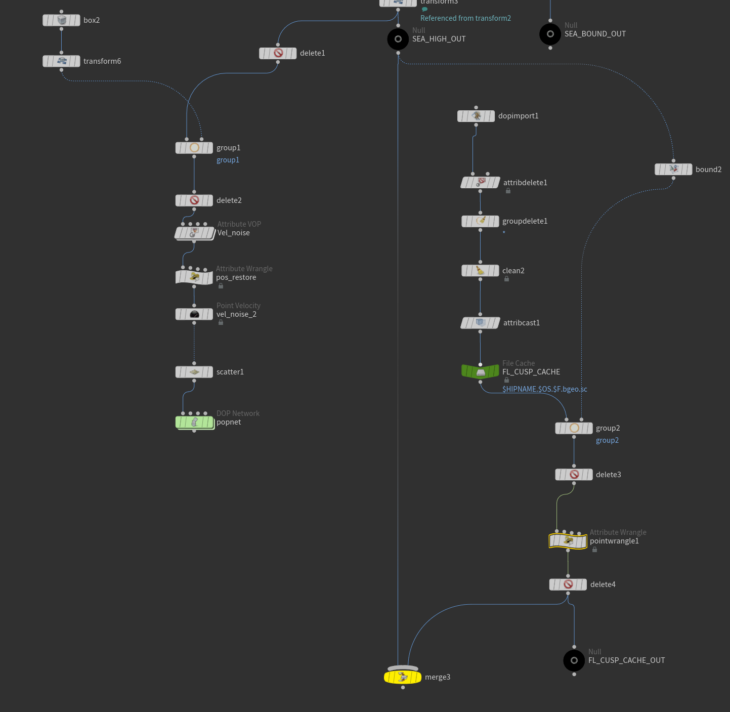
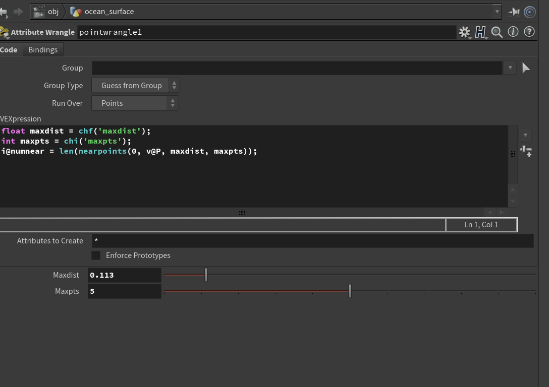
(Camera-based grass LOD optimization)
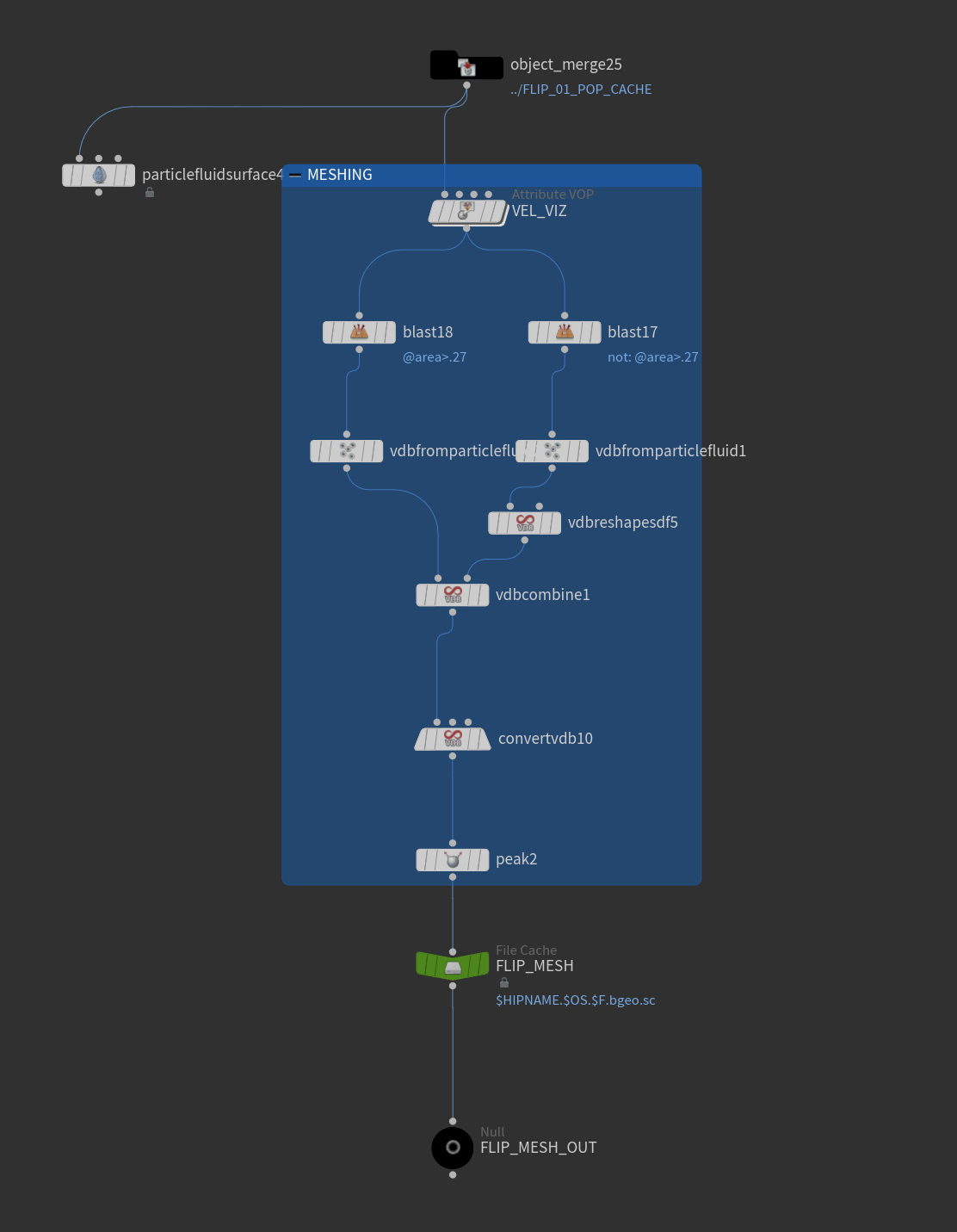
(Ocean foam on surface optimization)
(HDRI Background projection)
(Add rain footage)
Its been almost a month for a lot of updates that come with my thesis progress. Since I was busy with my summer internship during the past two weeks, I finally have time to update my blog today. Plenty of new modules are added to my project, and I'd love to discuss them.
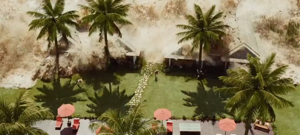
First, most dynamic trees in the scene have been updated using Speedtree trial version and simulated inside with random force applied. The "sample palm" file provides a very basic palm tree model but has some excellent textures for the later rendering process. Speedtree offers a "random" option that allows me to generate multiple versions of trees in a very short time. But the question is the way to export the cache. By default, Speedtree will export the model with FBX animation, and Houdini will recognize the animation as a CHOP network. However, I had experienced many unstable situations while Houdini randomly crashed when I tried to play the timeline, so I have to find another way. Alembic format helps me maintain the UV layout and animation when imported into Houdini, and it works just as it should be. The only disadvantage of this method is that alembic caches store all the animation in a single file while it is not space-friendly for the hard disk. Approximately 240 frames of the animation will generate 1GB caches per file. Inside Houdini, I use the "SpeedTree importer" module that comes with the software, which will read the cache correctly with shaders and animation. Here is the flipbook for the dynamic trees in the first shot. Other trees are static for now since I have planned to use Quixel simple motion node to offer them a procedural motion that will allow them to move gently with the wind force.
SpeedTree viewport
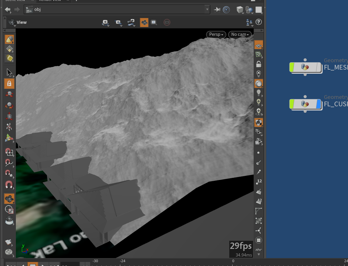
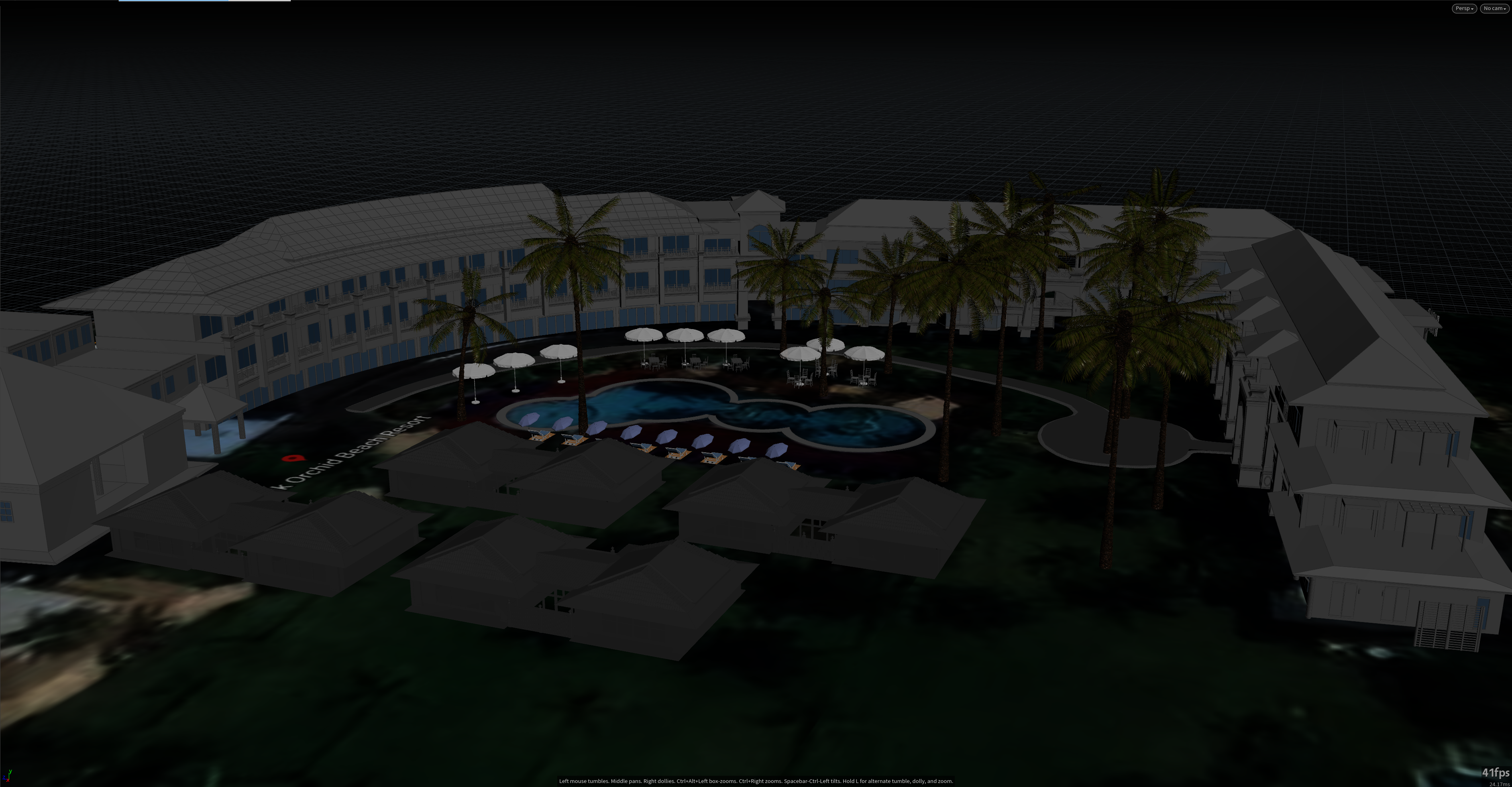
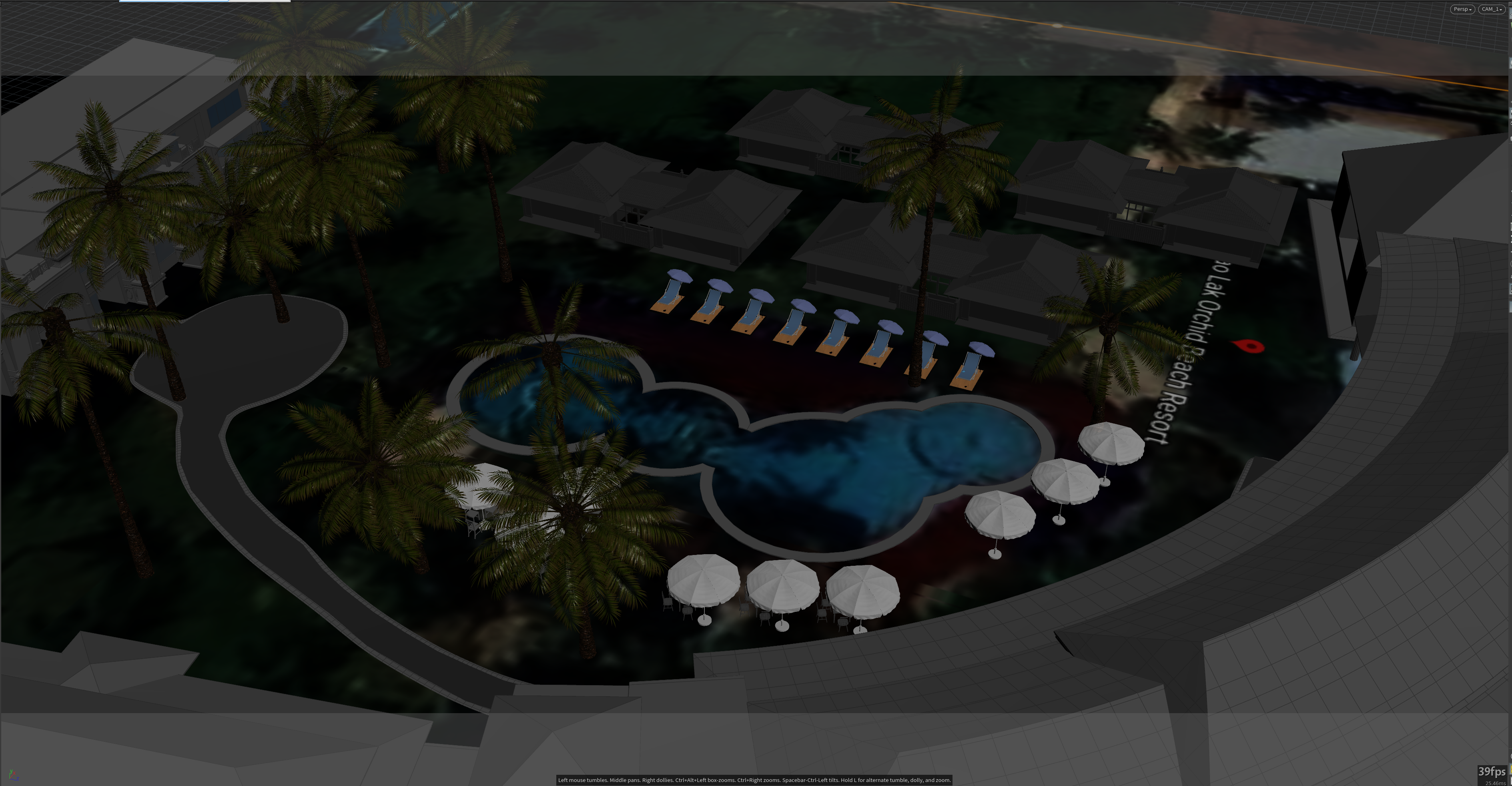
Shot 01 overview with dynamic trees
About foliages in Shot02, they are mainly from Quixel Megascan library. Megascan provides many formats and LODs that can be imported with textures applied, so it is convenient to place them based on the layout of my scene with the "Labs pick and place" node. It packs all the incoming geometry first, and then you could manually place them on the collision geometry in a custom way, so you could have unlimited control for a quick placement. Thus, I created a basic foliage layout for one bungalow using this node at first, and I could copy and paste them to other bungalows. Furthermore, they will have simple motion as well in the next update.

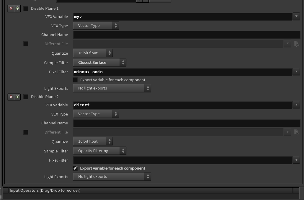
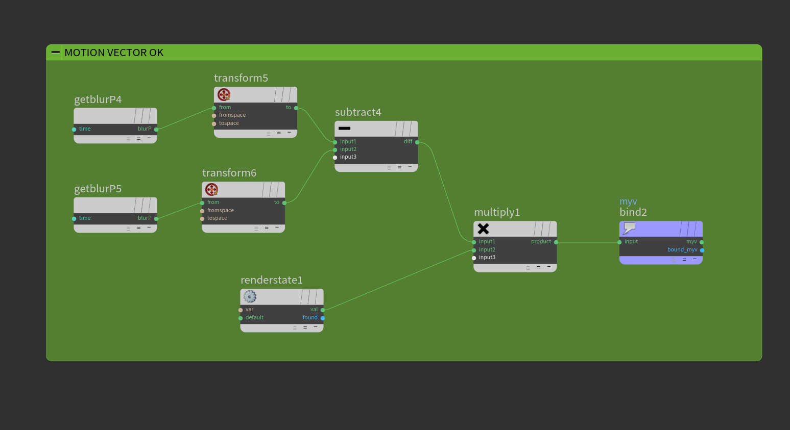
I have found a very useful thread talking about Mantra Motion Vector AOV, which allows me to have better control over motion blur inside Nuke, similar to the Arnold workflow. https://www.leoanka.net/motion-vector-houdini-mantra, and this page also shows another way of doing this: https://lewisinthelandofmachines.tumblr.com/post/159532447318/houdini-2d-motion-vectors-from-mantra. Basically, the shutter time controls how much the motion blur lasts, and that's why we need to compute camera space information per frame. So the whole process here is converting "current space" to "NDC" space and then applying a custom AOV layer with render state. Remember to disable the "Allow Image Motion Blur" after enabling the "Allow Motion Blur" option, so the diffuse layer will not be affected.
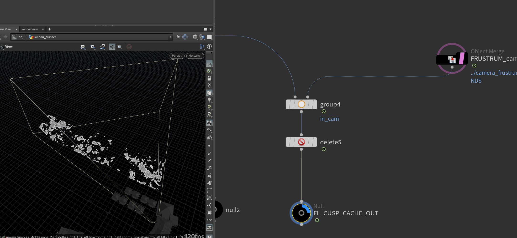
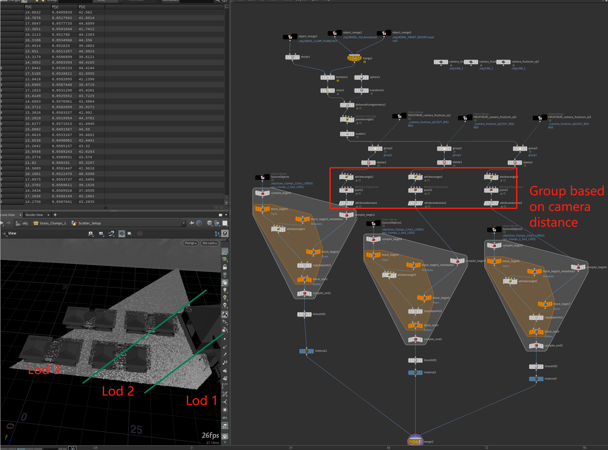
Let's discuss the LOD optimization that I did to the grass in the Shot02. Grass geometry is from Megascan Library, also with multiple LODs imported. Since I want to create more geometry instances in the foreground, it's necessary to have more points scattered in those areas. The solution is the camera distance. To achieve the density variation, I created a target object at the camera position and then calculated the distance in the surface plane point, which stores the value in an extra attribute that could be used later in the scatter node. After that, I created different groups based on the distance also and applied various LODs. As a result, it helps maintain the foreground details while saving some RAMs dealing with extra amount of instances before the render actually started.
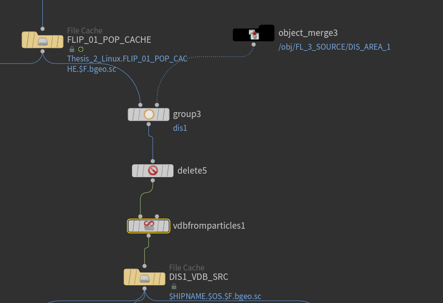
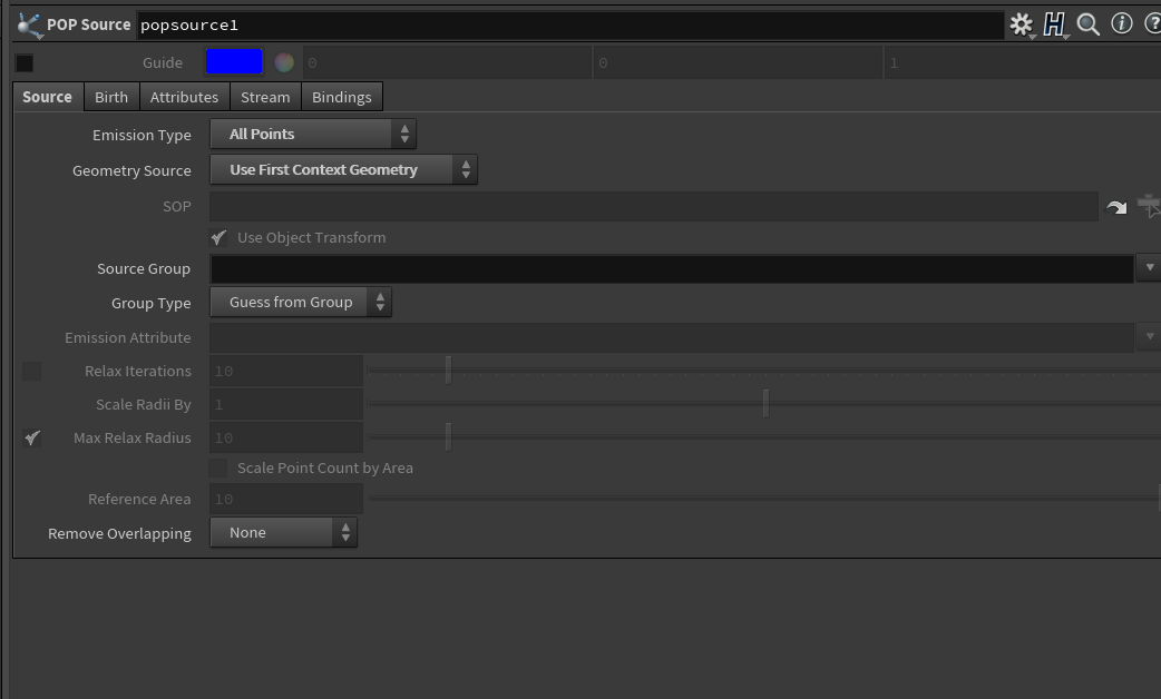
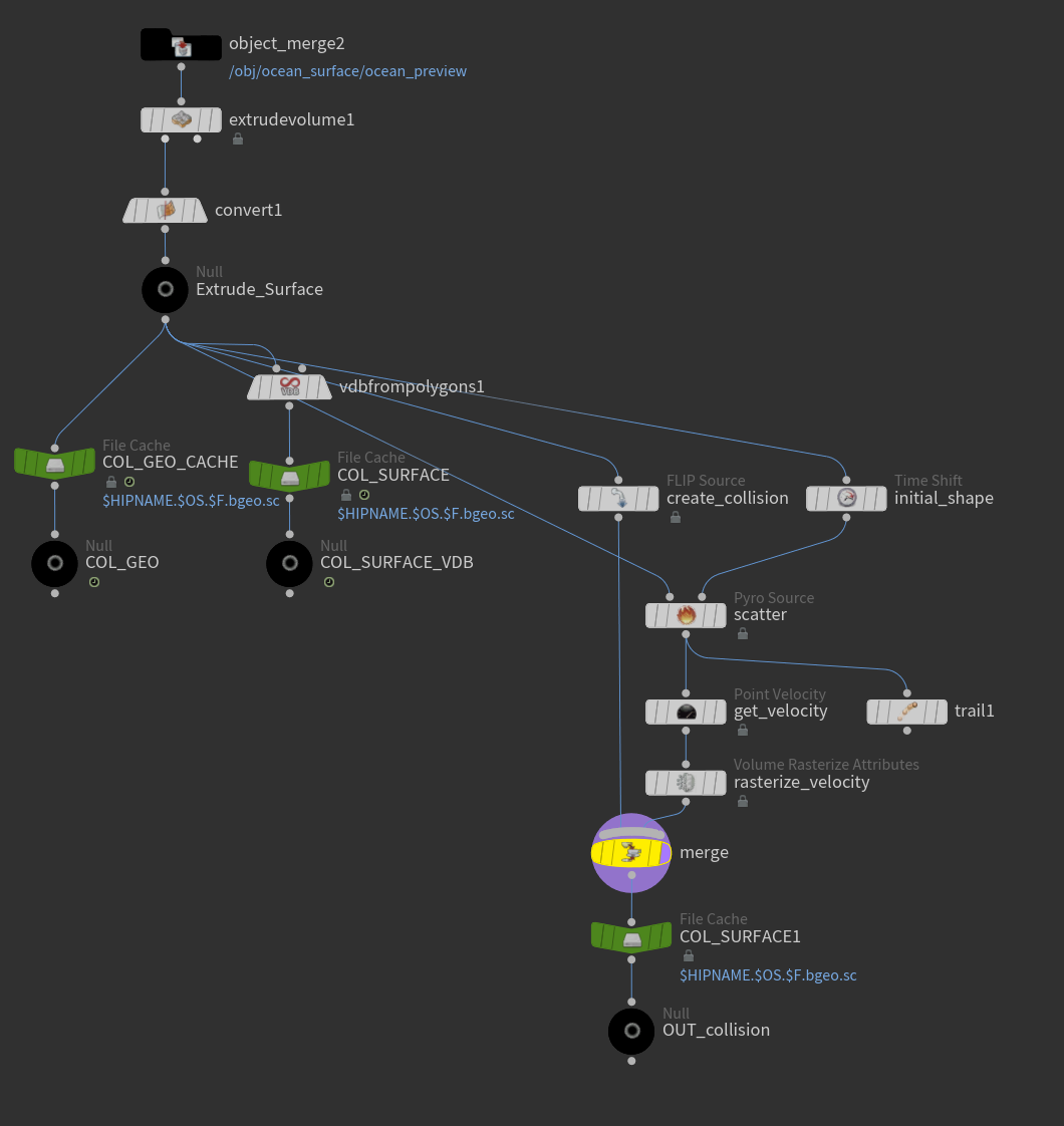
The same camera culling was used for ocean foam source generation, so the source will let the pop simulation only appear inside camera bounding. I used the pop network to simulate the particles floating on the ocean surface, which will finally be rendered as the "foam," and this method is better than the default "ocean foam" node because the pop network provides more artistic control inside the simulation.
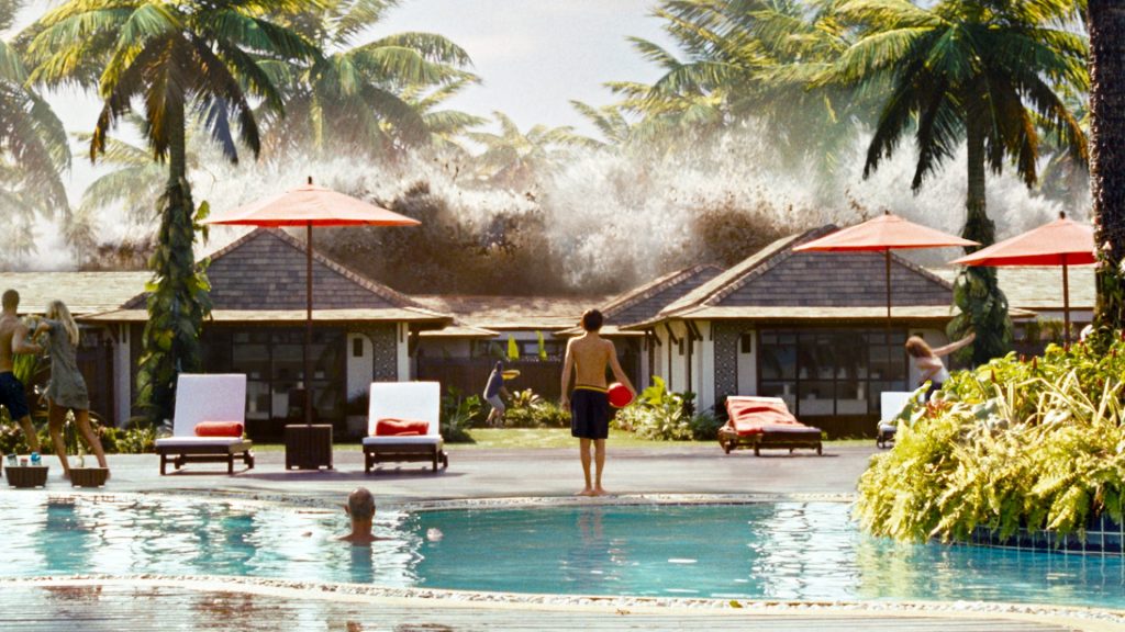
Inside Nuke, I did the camera-based projection using an HDRI that from CGSkies. It is a website containing a bunch of detailed sky HDRI for purchase. I downloaded one sample file for free, and the resolution is 3000*1500, and it is already ready for use. The setup in Nuke is a simple camera projection method that turns the 2d plane into a 3d sphere background. While merging all the rendered layers, I also added some rain layers blending the foreground to simulate a rainy day look. They are very subtle but essential in achieving a realistic look. And here is the latest version with two shots combined together.

Latest rendered version
Update 06/27
(Tweaking RBD sims for the bungalows)
(Tree rigging with PDG wedging simulations)
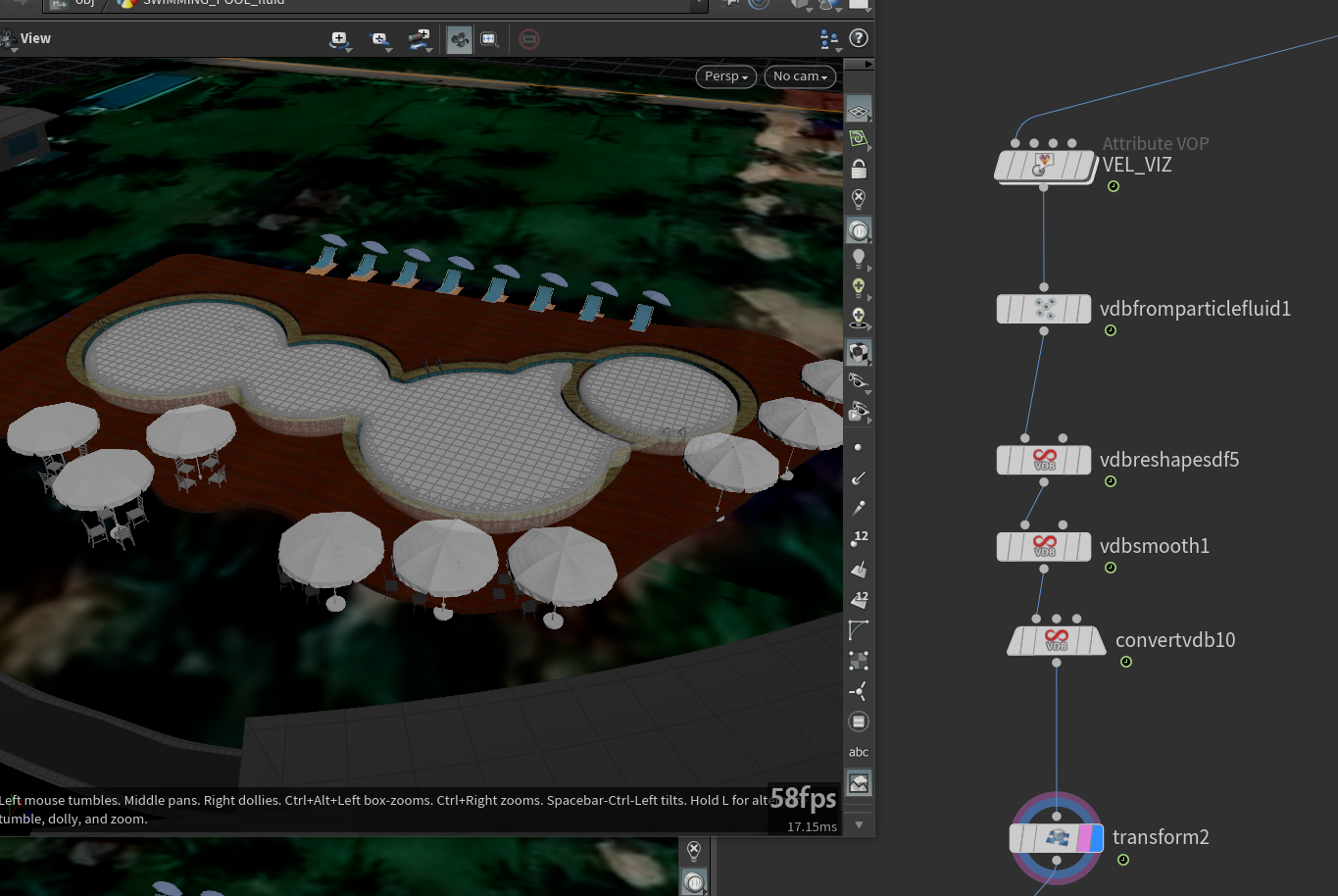
(Pool flip surface creation)
(Render tests for the trees/pool)
It has been a long time since not updating the blog…. And its because the internship took workdays' daytime, and there is not sufficient time for me to update the blog weekly after working on the thesis project. So this time, there are plenty of updates that I want to address. During the last two weeks, I have been working on the RBD sims for the bungalows, adding active areas for the fence and rooftop. I also started to build a procedural way to rig the tree model, which could be driven through PDG and write multiple caches in the queue without manual control. Furthermore, I have modified the pool model for generating a water mesh filling it using the flip solver. Then I have rendered some stills and also run some flipbooks to see the combination of those elements.
For the RBD simulation on the bungalows, based on the former RBD template, I have fractured the front rooftop and fence using different pre-fracture patterns. Since the rooftop is formed mainly by concrete in this example, I used the "RBD Interior detail" node to add displacement detail to the inside face group of the fractures by increasing face division. The wood pre-fracture shape is more reasonable for the fence because woods are easy to be broken along the vertical direction. And the most common way is the scaling trick – to scale it along the Y-axis before fracture and make it thinner, then scale it back. So the size remains the same, but the pattern has been stretched.
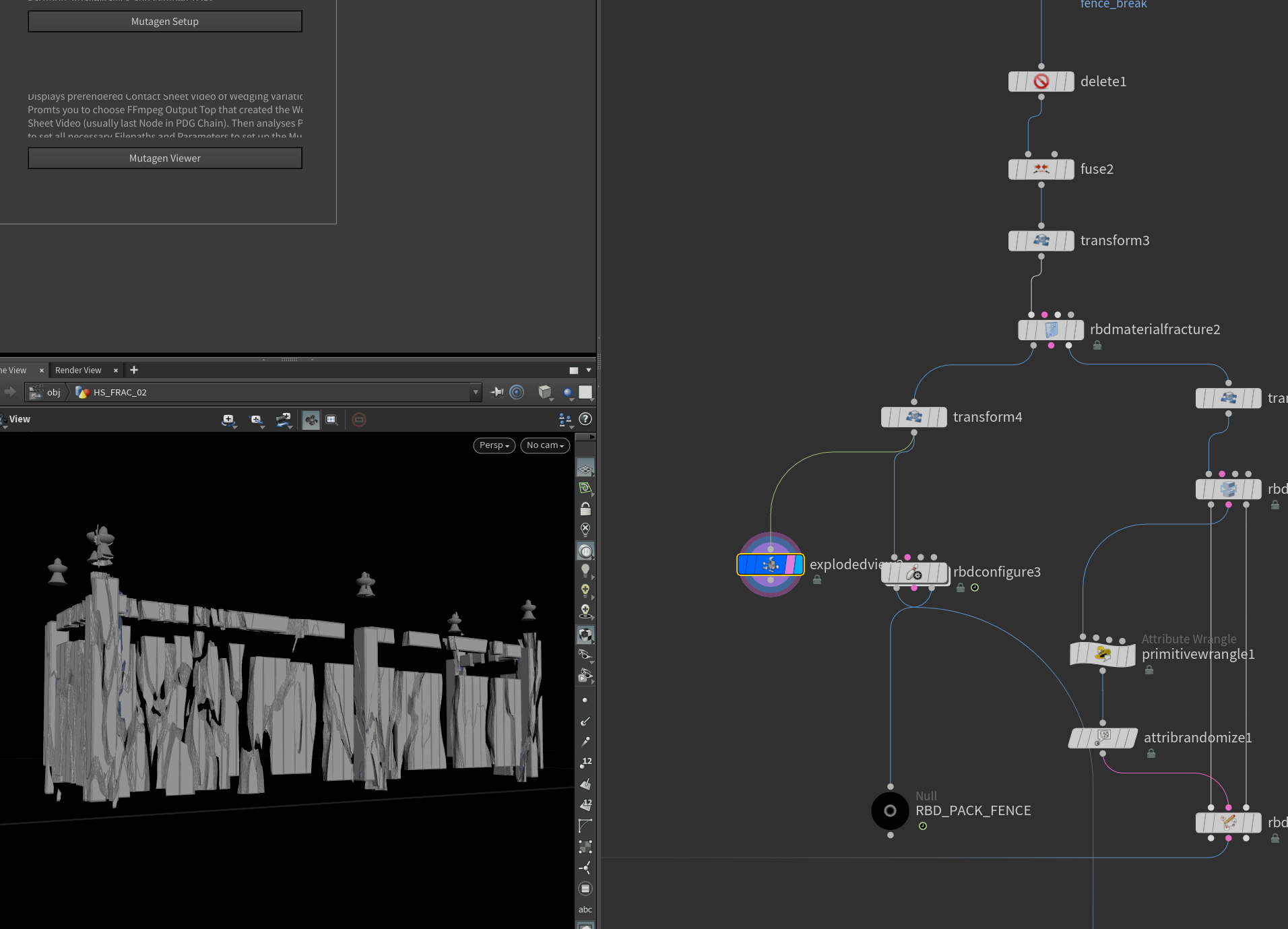

Here is the latest version of the RBD simulation with the flip surface. You could see the impact coming from the water surface resulting in the destruction, but they are not directly interacting with the water. Instead, the flip simulation generated a vel field that could be applied as an external force for the RBD sim. And the fractures could have the initial speed once the force field starts to influence them. But it needs to tweak more to gain a definitive look.
RBD sim with flip impact
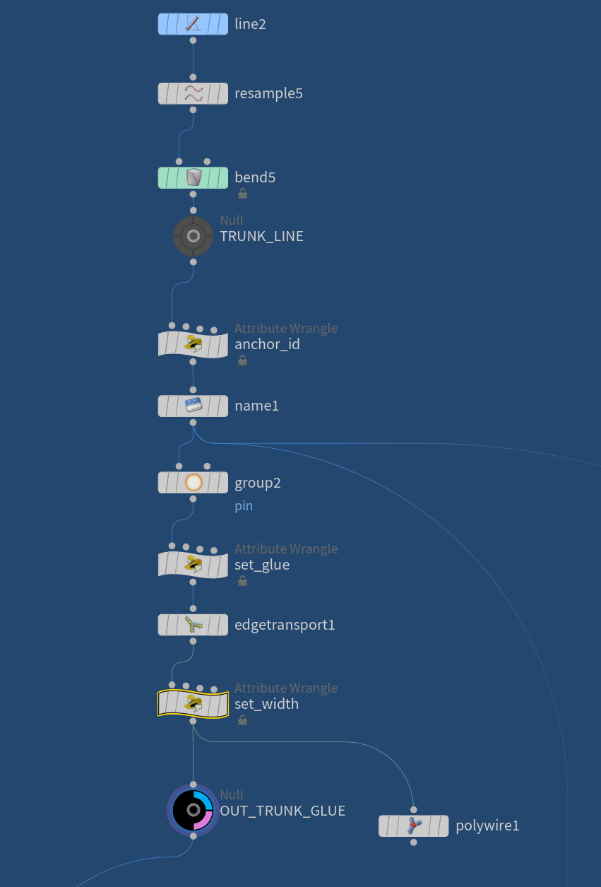
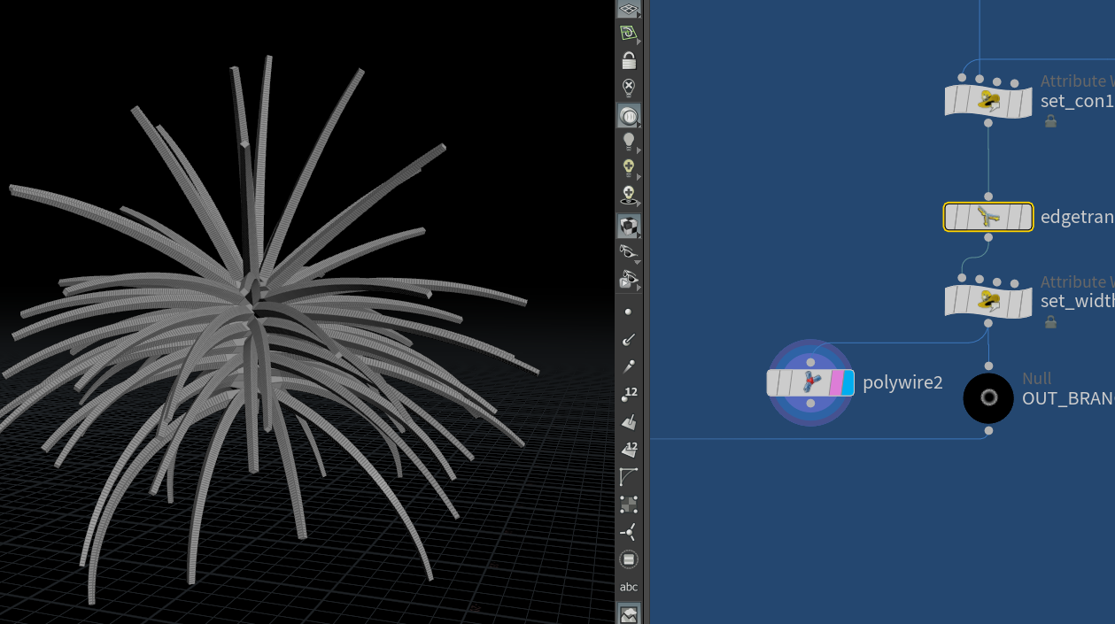
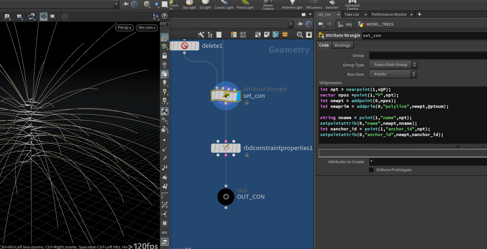
Then, I will start to talk more about the procedural tree rig. Starting with the trunk, the guide curve for the trunk is pretty straightforward – a simple line. The whole method is based on the wire solver, so the line needs subdivision to ensure enough points to calculate the dynamics. After that, some points are selected to become the "pin" points, which are static during the simulation. Wire solver requires the attributes called "anchor_id" to identify the constraints position and the name attributes on the point level, and they both need to be created. The "Edge transport" node calculates the distance from a certain group to other parts of the input geometry, so I use this node to generate the value for the width attribute, and it will tell the wire solver how wide the input guide curve during the simulation.
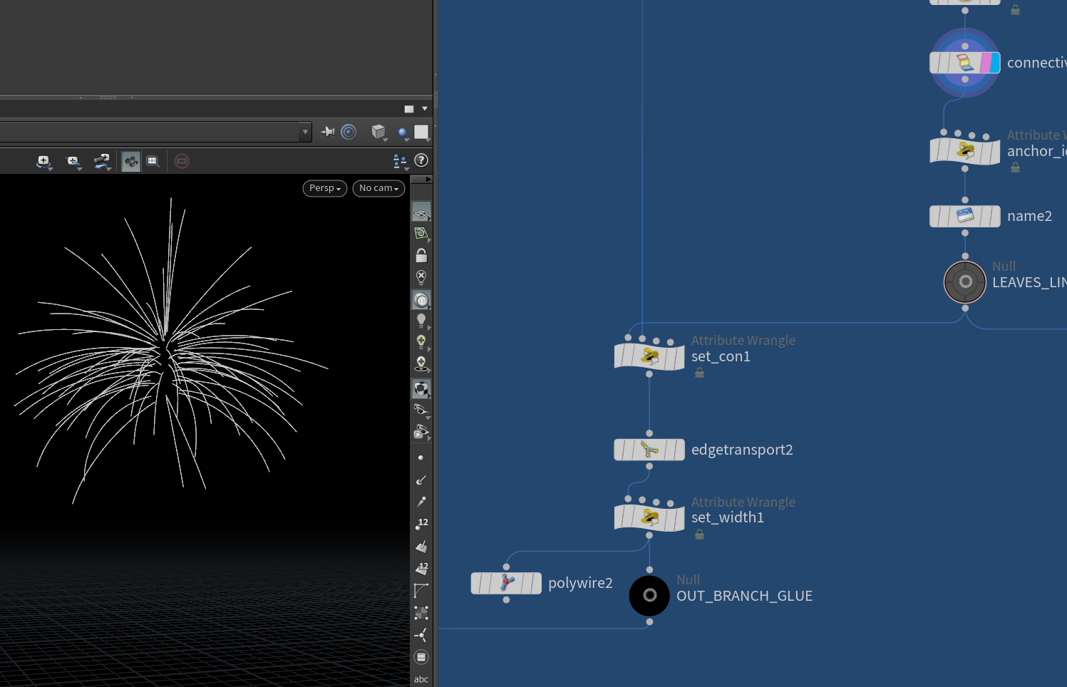
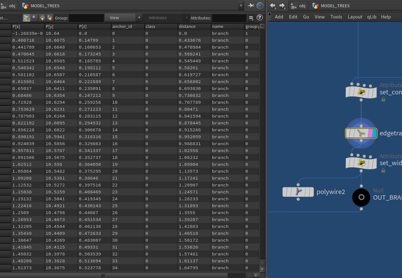
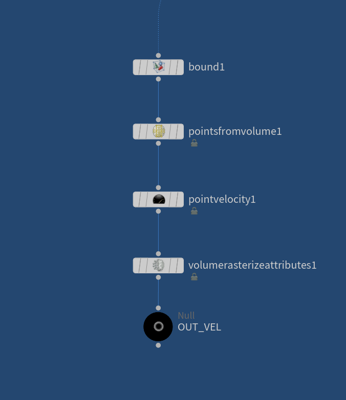
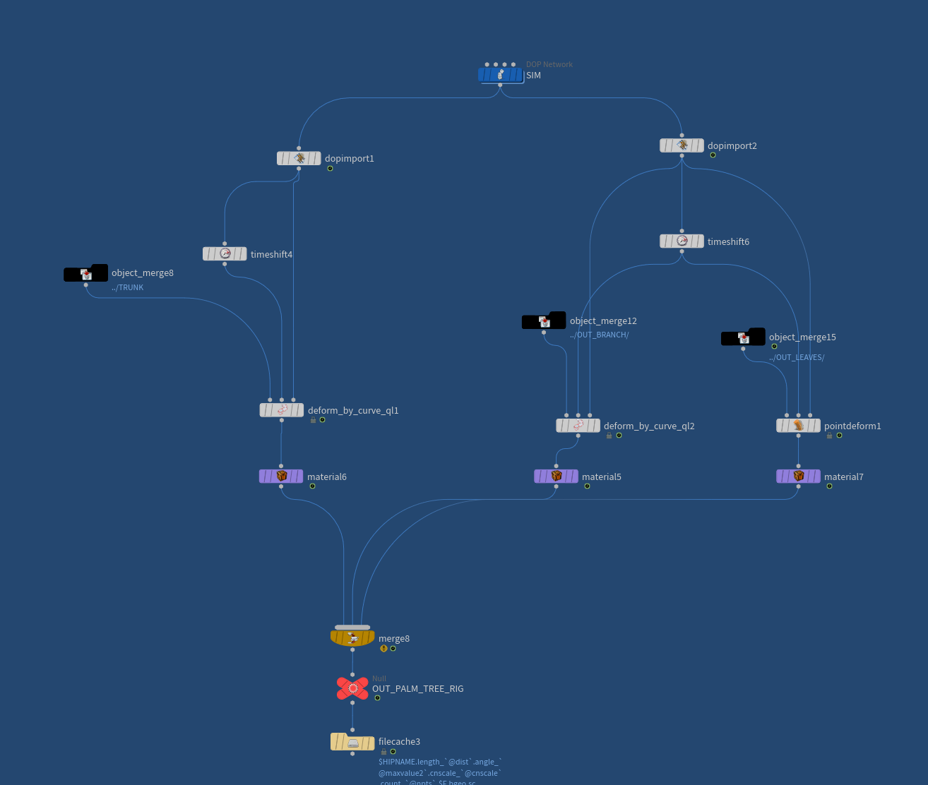
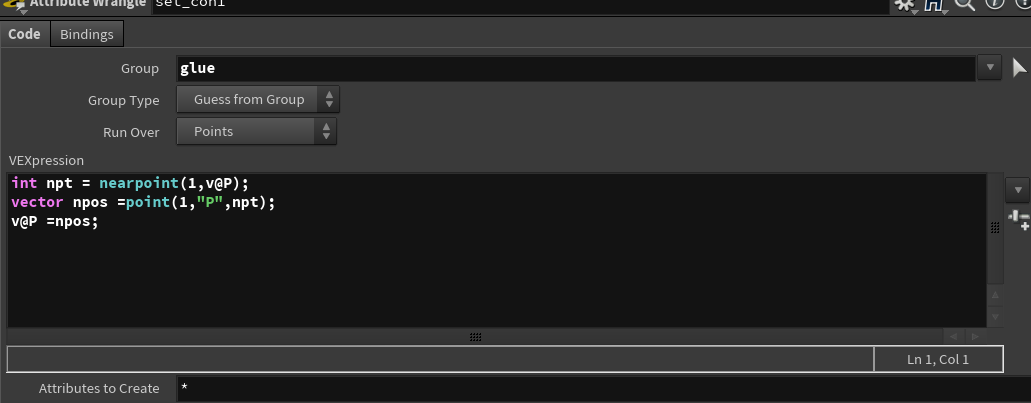
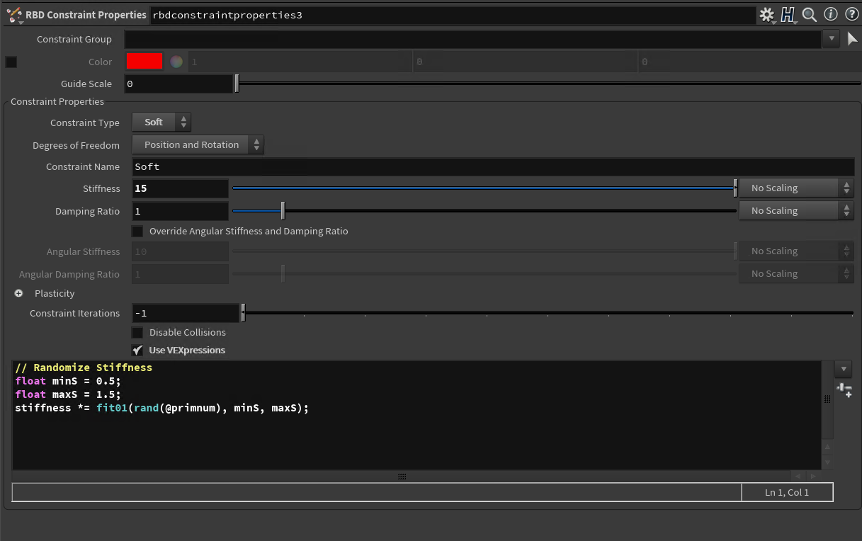
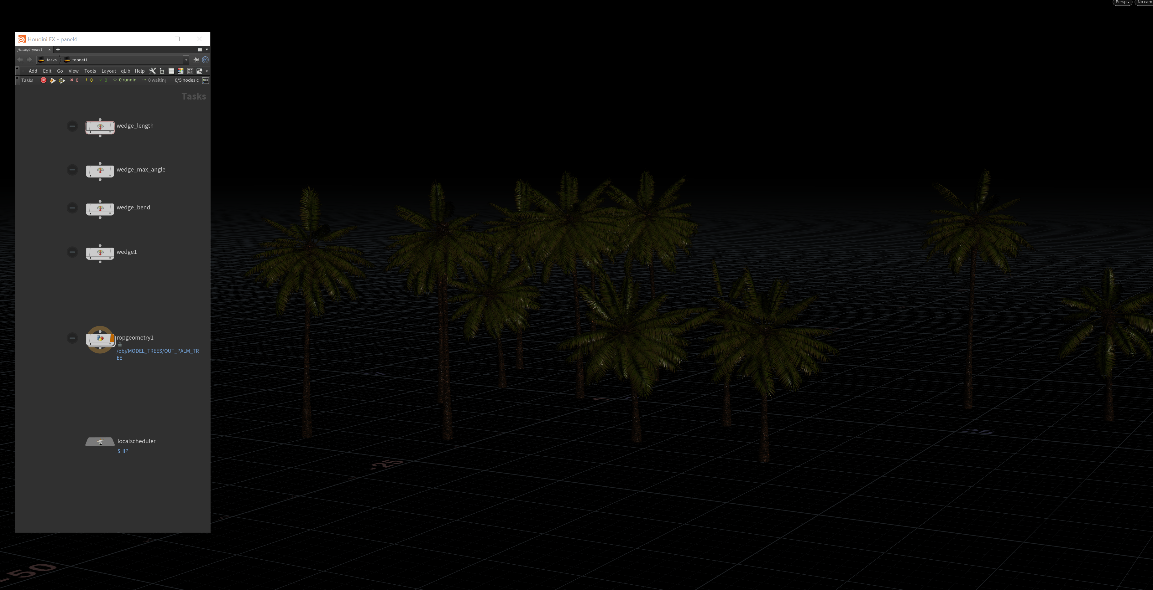
For the branches, the preparation for models is similar to the trunk part. Guide curves are extracted and put in an individual group, and then applied different anchor id and name attributes. Now it's time to set the connection between these two parts – the trunk and the branches. Using the point cloud, I could determine the point group with minimal distance between the two parts and add a primitive to the group. The result becomes the hard constraints group. Because they are similar to the RBD constraints, I could use the "RBD constraints property" node to set some basic parameters to the constraints and then apply them to the wire solver. The simulation definitely needs an external force field, so I create a simple directional velocity field through the "point velocity" node. Basically, the bounding area will be filled with points with velocity and converted to volume source for input. The guide curves will transfer the motion data to the original geometry by using the "pointdeform" node. Eventually, all of these simulations will be called in the Top network through wedging process. The wedge parameters can be added with preference, specific the length of the trunk, and the wind noise intensity, or the number of the leaves. Once the PDG starts, It will write multiple caches to the disk in separate folders bases on the wedge paths.
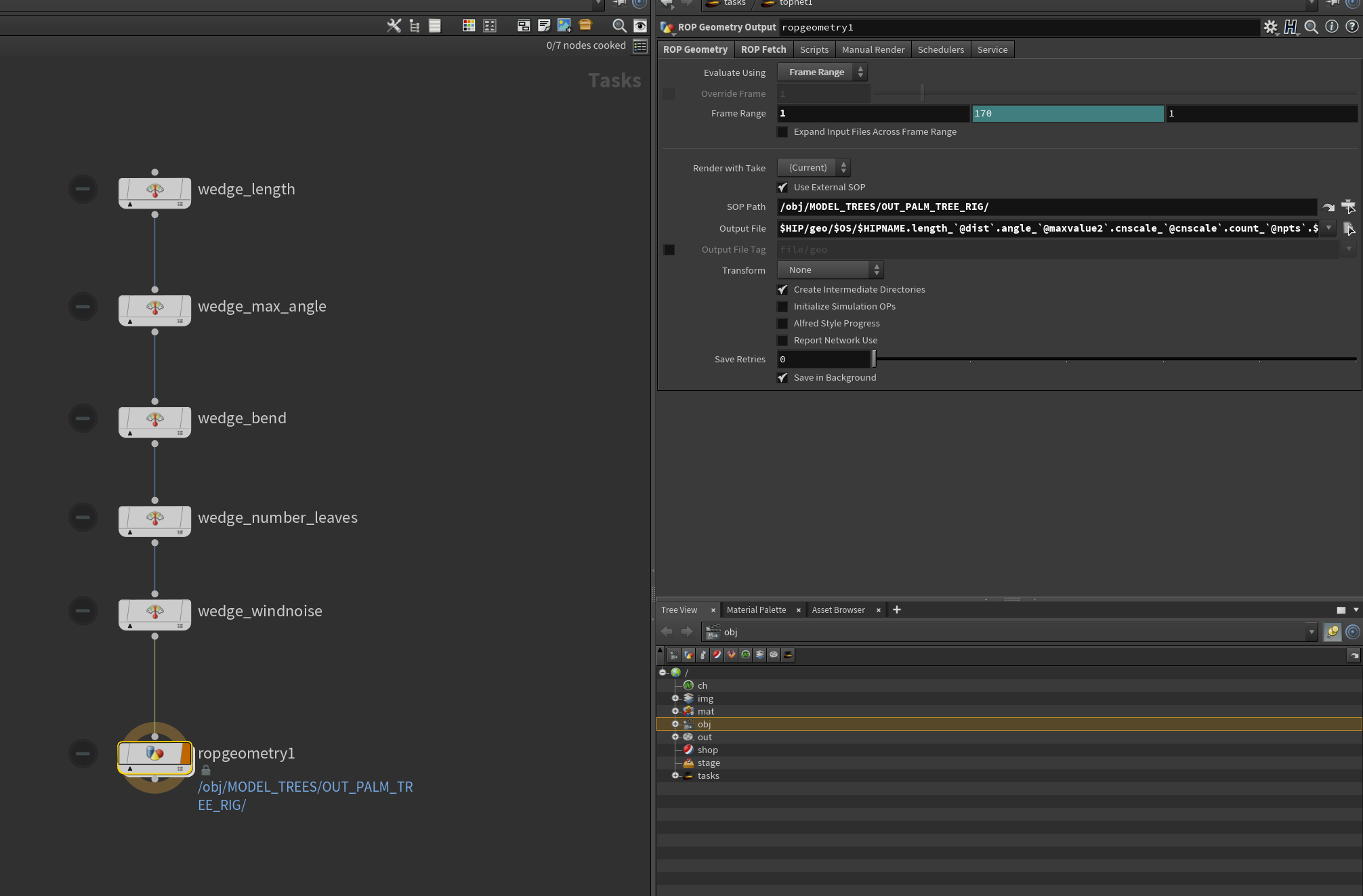
Multiple tree caches
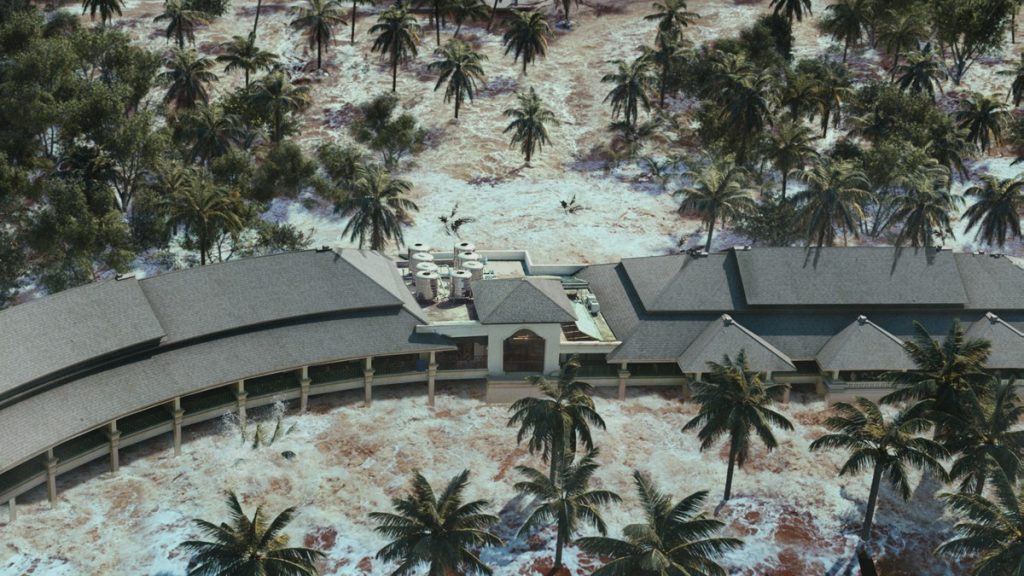
For the pool models, I created three primitive groups for materials, also save some space for running the flip simulation by extruding depth under the ground level. The water simulation in the pool is much simpler than the primary tsunami simulation, and it only requires a flat surface with subtle movement. As a result, I created an ocean spectrum with slow-moving speed and attached it to the ocean shader. Notice that the mesh for this simulation needs to be much flatter before the shader displacement because from the camera perspective, it is very challenging for the audience to notice the water surface movement. And here is the first rendered version for the pool simulation. Apparently, there will be lots of specular areas because of the shader displacement on the water surface.
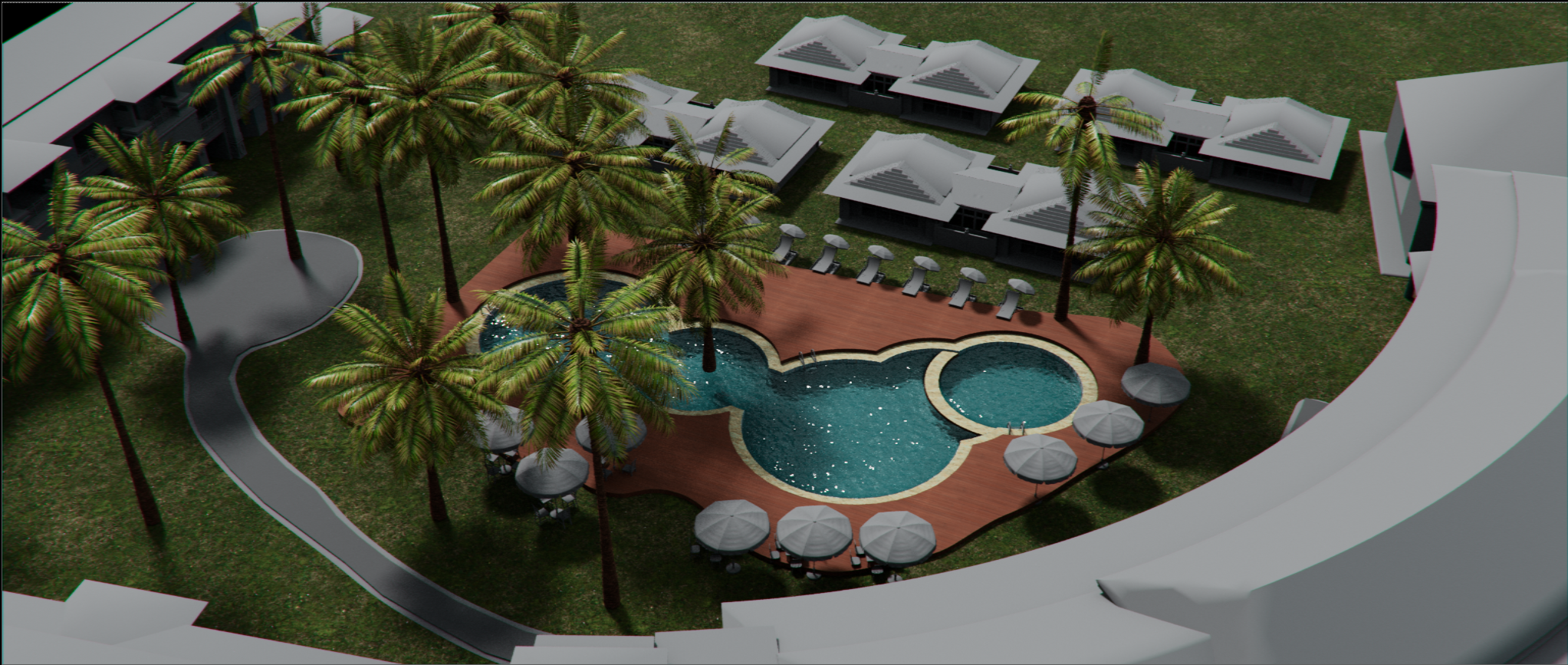
Sequence render test
Update 06/08
(Render the whole sequence with Whitewater)
(First pass of RBD Fracture)
This week, I started to fix the ocean foam displacement issue along with the ocean surface, also managed to render the whole sequence with a modified whitewater shader. Meanwhile, I started to pre- fracture one bungalow that will be affected by the flood impact.
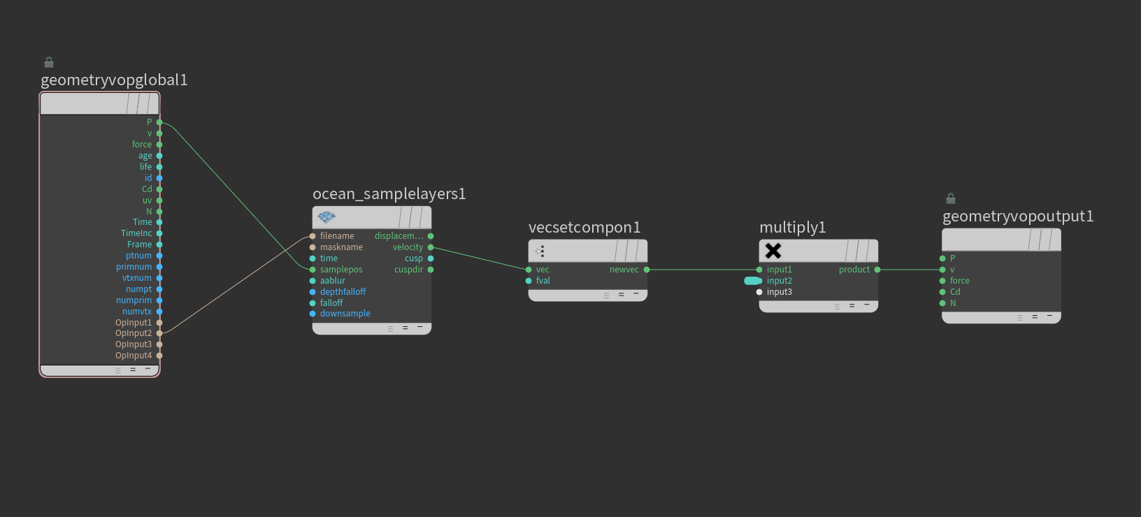
First, the ocean foam shared the same spectrum with the ocean surface initially. Since I made a few changes with the noise of the surface and custom modifications, the foam layer should be applied to those changes also. Here comes the first problem: the foam layer should be displaced in the geometry level after those changes. Due to the nodes' orders, the displace node has been put to the end using the “ocean samplelayer” node inside vop network, applying displacement from the ocean spectrum. Then, the result has been separated into two different render categories: one is rendered as pure volumetric puff look, and another is rendered in particles, combined inside Nuke then to have a more dense foam style. Particles do have scale attributes, so I used the particle age, and life attributes to decide the scale attribute. Then, I deleted some particles based on the points neighborhood distance and using the “point replicate” node to increase the total amount.
Rendered sequence
Ocean foam generation process
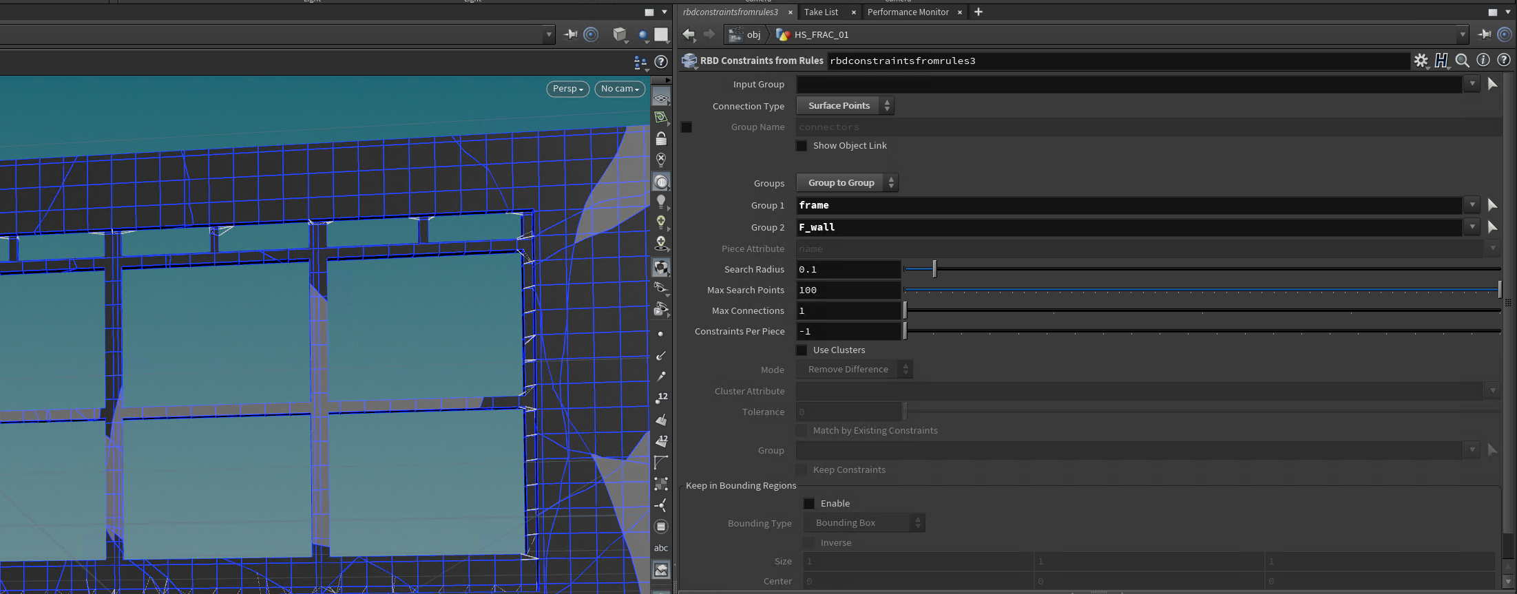
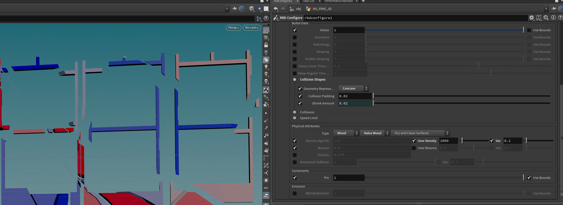
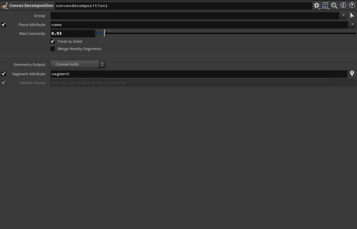
Then, I started to pre-fracture one of the bungalows. Since the bungalow has different groups during the making process, I could use the group to identify which parts need to be broken. This time I have decided to use the new RBD fracture workflow – some new nodes are coming from the 18.5 version – to speed up some basic RBD settings like constraints type and pack attributes. I also want to mention the usage of the “Rbd constraints from rules” node. This node provides a handy function that allows users to choose constraints generation based on group type, meaning I could easily generate constraints between two groups without manually adjusting input constraints names. I used the RBD Convex proxy to generate an approximate shape proxy of the original ones for concave objects. The proxy participated in the simulation rather than the high-poly source, which saves simulation time, and the proxy overrode the default convex proxy inside the dop network. Most of the constraint types are soft constraints except the connection between the front wall and the ceiling. Here is one playblast for the most recent RBD dynamics with the flip mesh; the tiles still need more impulse at the contact areas.
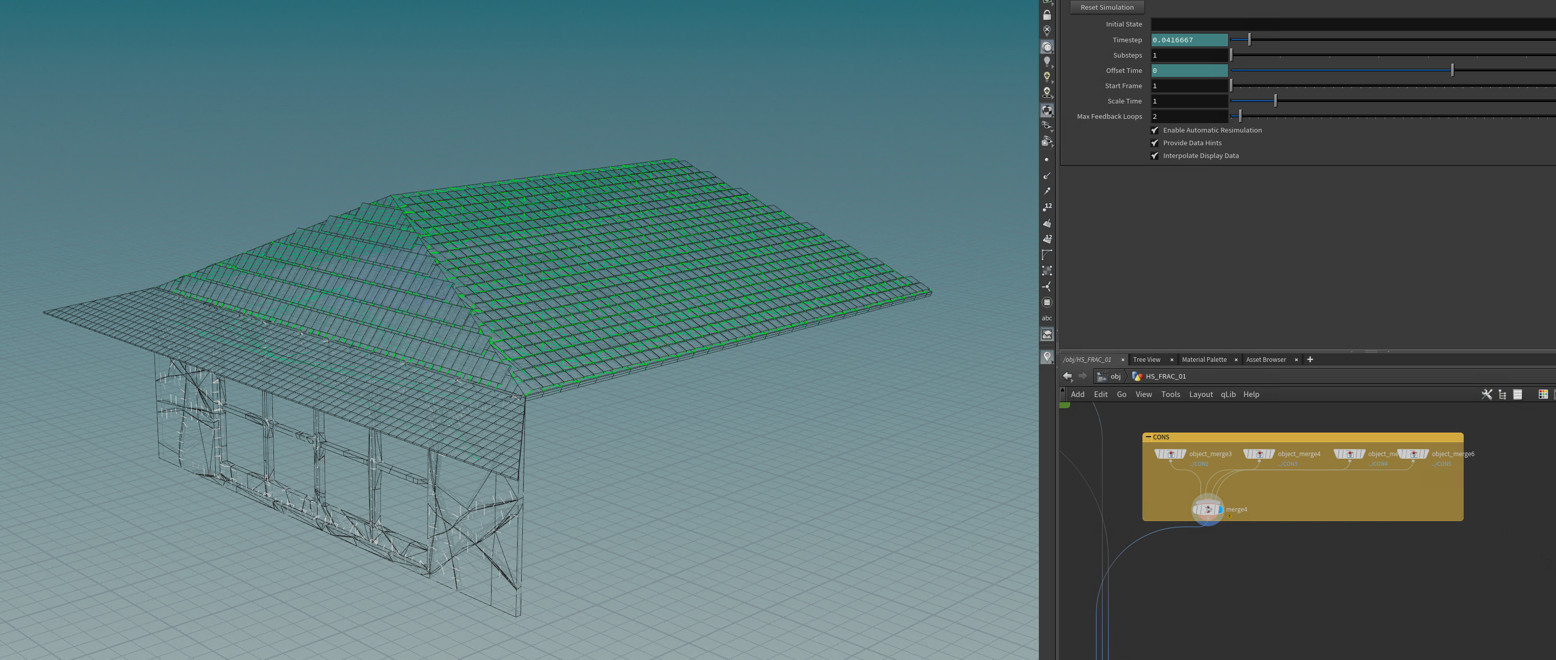
RBD simulation with flip mesh
Update 05/24
(Multi-layer rendered)
(Whitewater rendered method update)
(Material updated)
This week, I researched the proper way to render flip mesh and whitewater for the closed-up shot and rendered part of the sequence with render layers added to test the pre-compositing. Also, I have added more displacement details to the ocean surface by adding one more ocean spectrum for the ocean material.
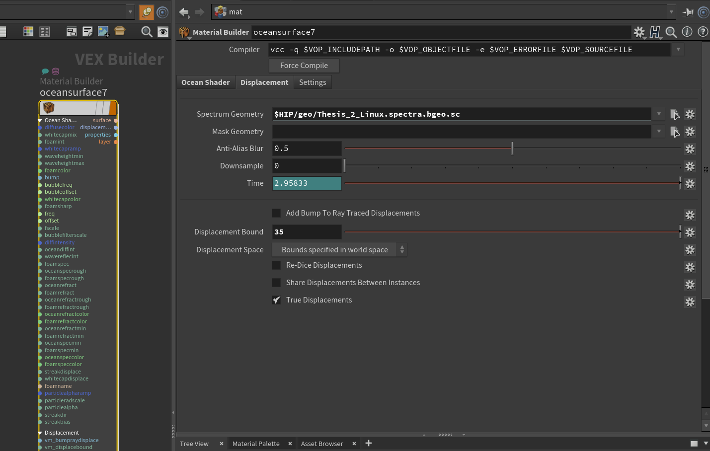
The ocean surface now rendered with full displacement based on the cached ocean spectrum geometry. The last time when I rendered the ocean surface, I gave some subdivision to the geometry and rendered it with deformation directly. However, some displacement details were missed because of the insufficient geometry subdivision. Then I switched to the default way – which is the correct method - to plug the spectrum geometry inside the ocean material, letting the material itself controlling the displacement details. Since the displacement in the material could reveal the maximum resolution of the cached ocean spectrum geometry, the final rendered ocean surface could be rendered without subdivision issue. In this way, the ocean mist also needs to displace to match the ocean surface's position.
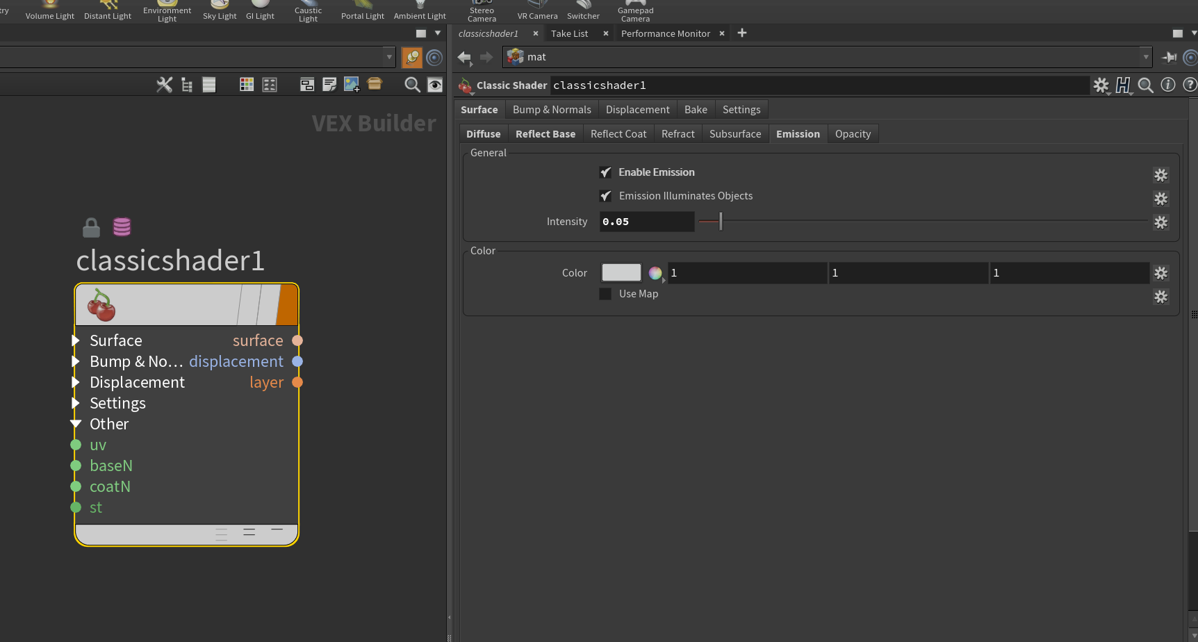
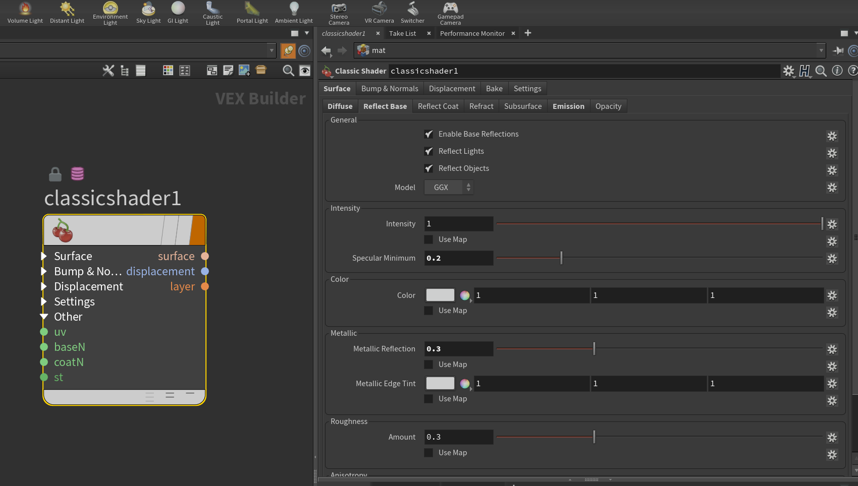
For the whitewater material, converting whitewater into volume/fog works fine with plenty of shadow casting on the ground during rendering, but it lacks some details during the conversion. Here is the comparison with rendered sequence. You could tell that the left one is the volume version with great shadow in general, but it is blurred most of the time, and it seems the resolution for the whitewater is not enough to capture all the dynamics of the whitewater for the close-up shot. The right one is the version with whitewater rendered as pure particles with existed alpha channel and point scale settings. As you can see, most of the details are kept even with the motion blur added, specifically in the high-speed area. The particles have been assigned with the "classic shader". Inside the shader, the specular Minimum and the Metallic Refection have been increased to ensure the particles have enough specular, creating the "droplet" look with directional light in the scene. Meanwhile, adding a little emission also helps get a closer look to the volumetric style for the whitewater.

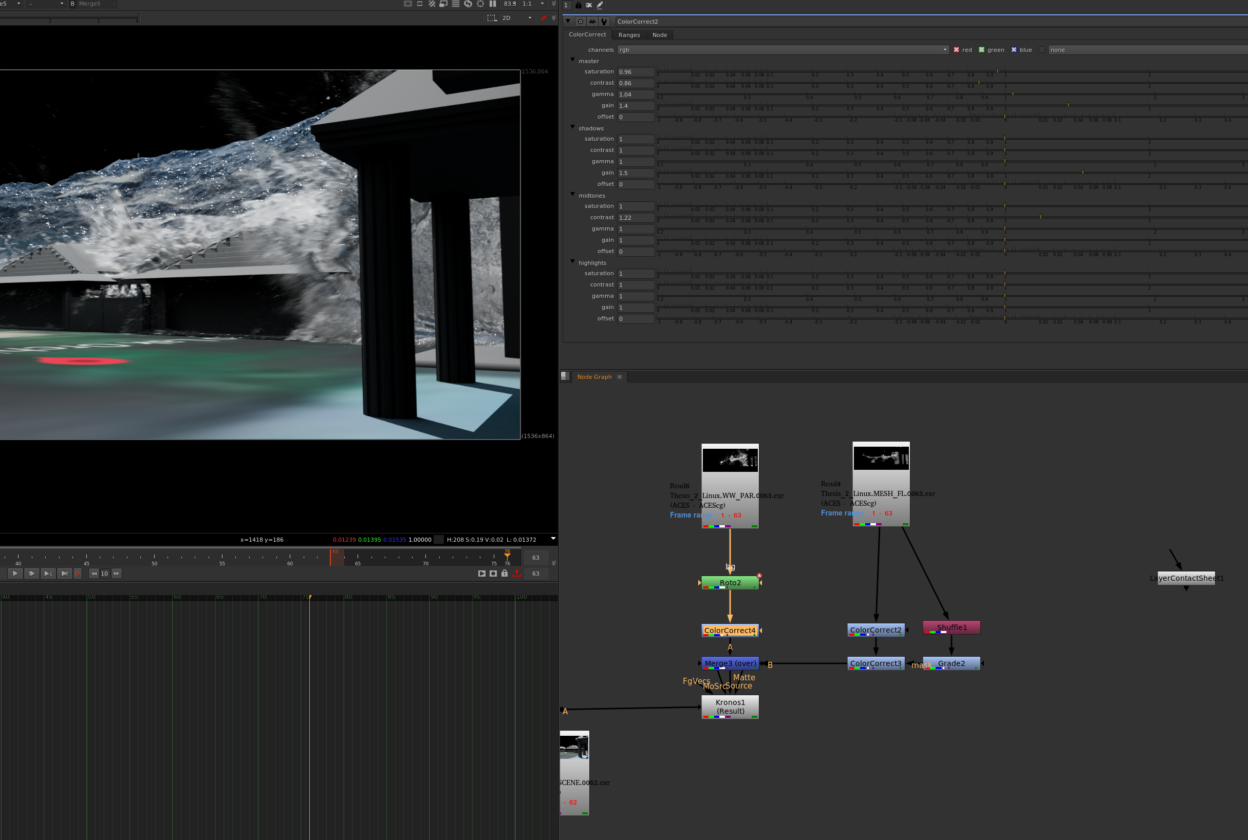
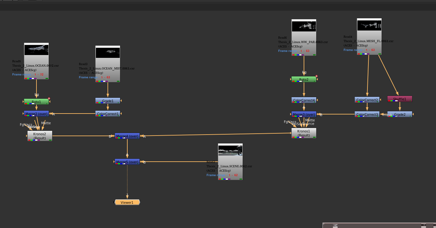
During the pre-compositing process, I assigned different motion blur amounts to the foreground and background layers and color-corrected the flip mesh to make it less saturated in both shadow and mid-tones. The whitewater looks a little bright to me under the current light condition, so I have decreased the primary intensity as well. Finally, I have two different rendered sequences for comparison. Obviously, the second one with the whitewater rendered in particles looks better than the pure volumetric one.
Sequences comparison (More frames will be uploaded soon)
Update 05/16
(Extended the water sim to cover more areas)
(Flip mesh generation)
(Render test with flip mesh)
This week, I have extended the flip simulation to the left to cover more areas within the camera, also trying to add small ocean details with particle simulation based on cusp attributes. There is a slight adjustment on the ocean material as well as the flip mesh material. And I also added more collision objects like the right building part to change the flip dynamics drastically.
First, there is not too much difference with the procedural node sets with the extended simulation part, as they require the appropriate bounding information about the sim area. So I have copied another bounding box to the left and use that to identify the whitewater and mist element boundary limitation. To clarify, my machine has almost reached the max limit particle counts when combining all the sims, so I have to decrease the particle emission count for both whitewater and mist for the extended area. For the new collision geometry(the right building part), because it has some open area such as window and main entrance door, instead of doing the simple VDB conversion, I have found its better to use the "clean" node first to ensure there is no non-manifold polygon existed. For the collision proxy, it's necessary to find the balanced voxel separation for the VDB, as it just needs to represent the general shape of the polygon.
Meshing particles could be very time-consuming since it will need the surface VDB information to generate polygon based on particle counts. The traditional pipeline for meshing particles uses the "particle fluid surface" node to generate the polygon. The node is a combination of custom VDB tools such as erode and smooth. However, the generation process is uniform for all the particles. If we want to keep as many details as we can in the mesh, the only method is to lower the separation value, which is inefficient. As a result, we need to use a mask to decide the separation for different areas. For example, in the high-speed area (splashes), the particle separation for the mesh could be lower down to increase the details in the final meshing. Other regions in small velocity would remain larger particle separation with adaptive polygon to speed up the meshing process. Then, we could merge them to gain a detailed look without spending extra time.
Mesh polygon flipbook
The ocean itself needs some whitecaps and streaks to reveal its scale relative to the buildings and bungalows. We could definitely go to the shader and increase the whitecap color value or the streak. However, another possible method to add extra details to the whitecap area is that it uses the pop solver to generate particles colliding with the displaced ocean surface, which could be very effective blending with the shader. Those particles are converted into volume finally to be regarded as the mist for the ocean surface.
Finally, I have decreased the refract value for both ocean and flip materials. The refractive value controls how much light bouncing through the bottom of the water, so the value's decrease could result in more depth in the final rendered images. As for the tsunami, this change will also help with getting a realistic look. The renders took a longer time for computing mesh with whitewater and water mist, and the render time reaches 15min for 720p per frame.
Update 05/10
(More separate whitewater & mist sim)
(Create whitewater & mist shader)
(First render test)
This week, I have continued working on refining whitewater and mist simulation on other areas and started to create volumetric shaders for both elements. Also, I have tested the render with a basic lighting setup to have a better pipeline for the rendering part of my project. The render time is not quite long as all the layers are in 720p; for example, the whitewater sequence took 6 hours for 120 frames, and mist took 3 hours.
For the simulation part, all the settings for other areas are pretty similar to the first completed simulation. Basically, I just need to change the bounding box location, and other nodes will automatically read those parameters and cache out the elements that I need. Notice in some areas, some particles have a large velocity that is not desired, so I have attached a “pop speed” node to limit the maximum speed during the simulation.
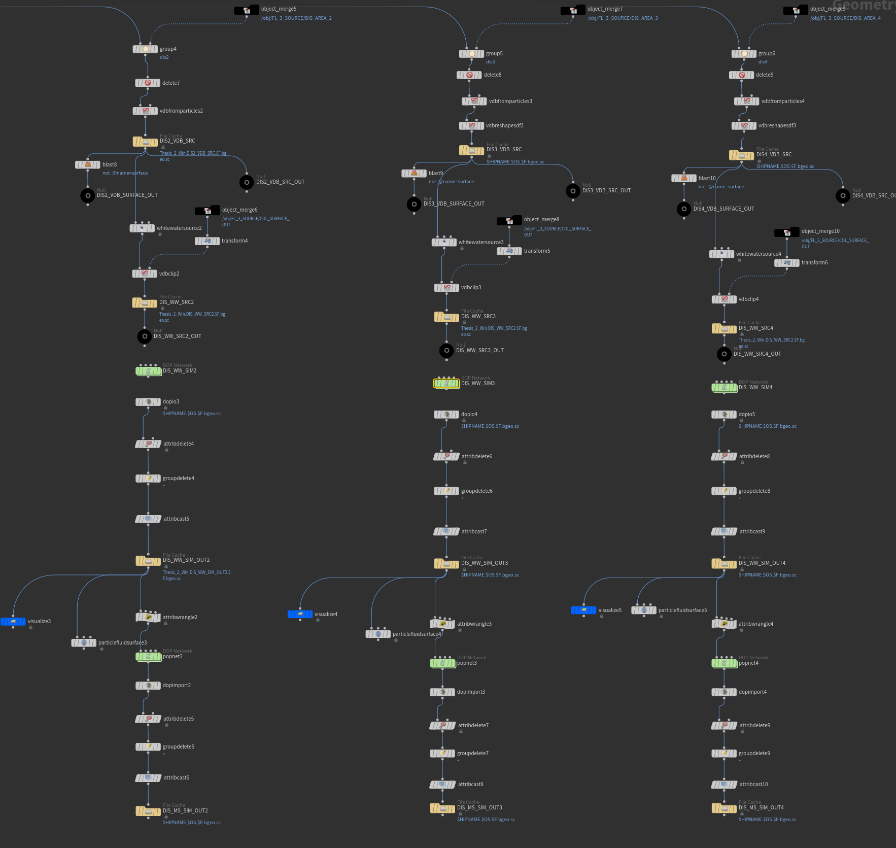
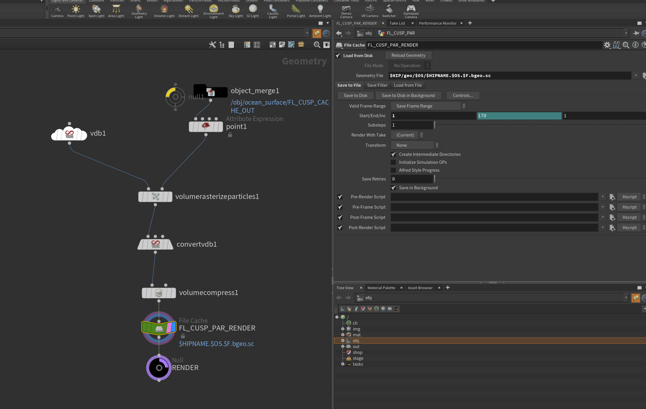
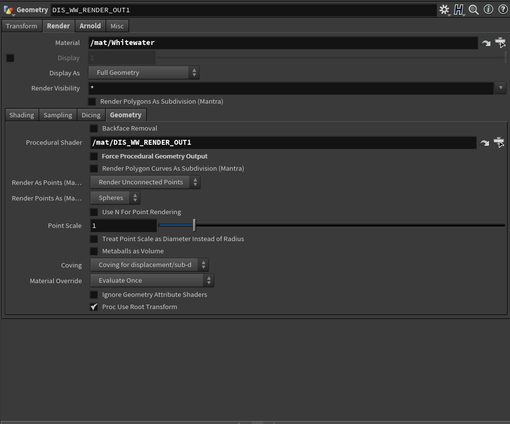
After finishing caching out all the necessary particles, it’s time to start thinking about optimizing shading and rendering. Since the total number of particles can get huge when merged, it will eat more memory during pre-render process (Loading caches and generating IFDs). In SideFX’s official documentation, one page discusses using the “Delayed loading procedure” method during the Mantra rendering process, which will force the Mantra node to read caches from the disk without processing the embedded geometry. Thus, the render time could be alleviated with extensive file rendering. https://www.sidefx.com/docs/houdini/nodes/shop/vm_geo_file.html https://www.sidefx.com/docs/houdini/nodes/vop/file.html
In the material network, the “Delayed Load Procedural” node read the caches that needed to be rendered, and then this shader is required to be assigned in obj level under the “Geometry” tab with “Procedural Shader” enabled. Mantra will start to load the procedural shader (the disk cache) during render time with other standard materials assigned. Possible bugs: This method will work most of the time on my machine with Linux system, but sometimes the Mantra node has error notifications popped up, showing segmentation errors after a few frames.
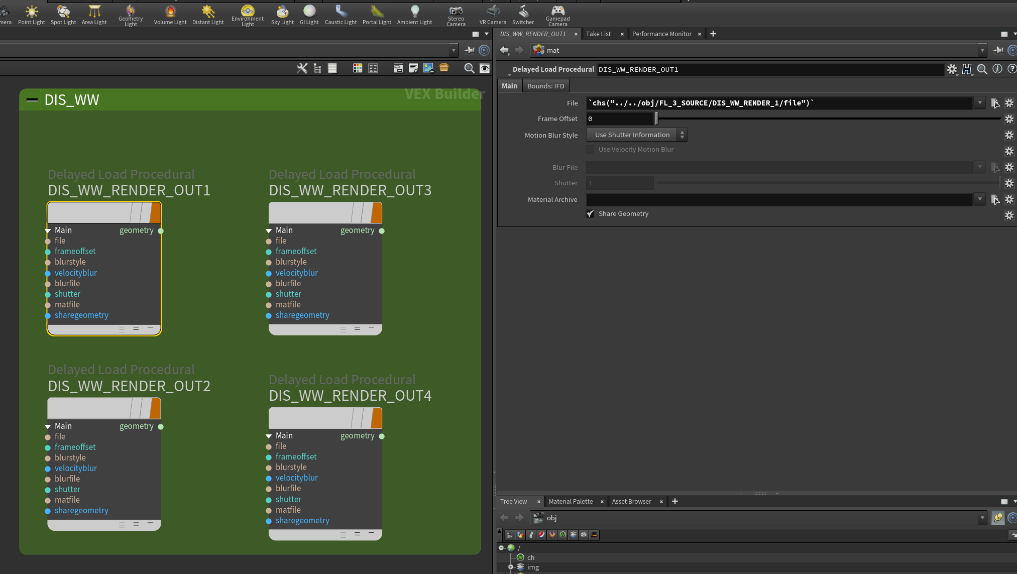
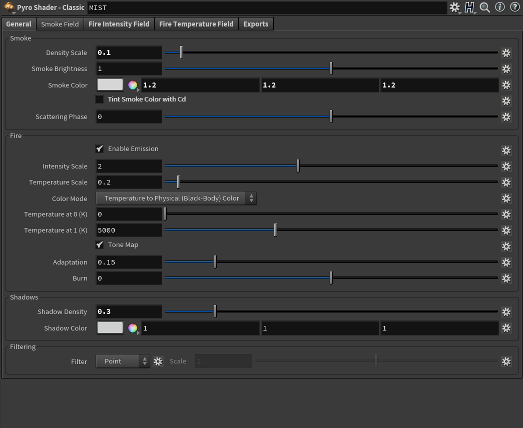
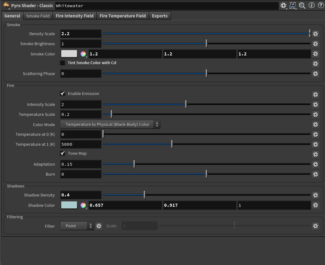
Whitewater and mist are two elements that need to be rendered in volumetric shape, so I use the “volume rasterize” node to transform the particles into volume. The volume voxel size could use the exact resolution as the simulation to keep consistency without scale issue. After that, I use the volume compress node to compress the volume cache stored in the disk to save space. For the shaders, I use the classic pyro shader in H18 – which is the common one for volume, and also, I need to do is tweaking the density and shadow on different elements. For instance, whitewater needs a heavier density than water mist, and the shadow is slightly blue rather than entirely white.
And here is the first render with whitewater and mist added to the scene. Some whitewater caches have camera culling from the second camera, and I am going to fix this issue by assigning different culling bound depending on shots. Also, I have noticed that the ocean surface needs more white caps on top to have a similar appearance to the simulated part.
Update 05/02
(Create whitewater separate sim)
(Create Mist separate sim)
(tweaking flip sim)
(Continue optimization of the cache)
This week, I started to add whitewater and water mist to certain areas for testing the separation simulation method. Since the scale of the scene is large, it is not possible to reach lots of detail by running a single whitewater and mist simulation on the flip with a single machine. So I analyzed the flip particle source that I have created last week and optimized a little more to emit whitewater and mist better.
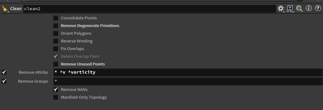
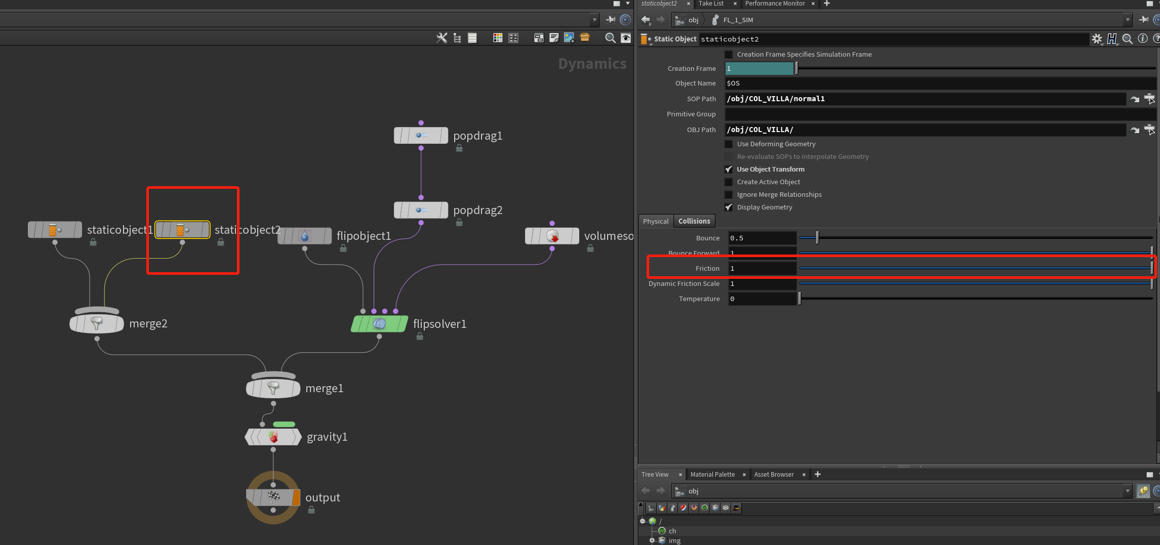
Inside the flip simulation dop network, the simulation area is controlled by a bounding box manually to limit the size of the simulation. Because the pop simulation for emitting the flip particles has already been optimized before, I could attach the exact sop solver to the flip solver again, deleting those flip particles intersecting with the ocean surface or behind the ocean surface. (Those particle numbers can be huge and slow down the computing speed) It is better to limit the speed by introducing different drags based on groups or simply delete them by range during the simulation with a sop solver for some particles with high speed during the collision with the bungalows. Notice that It is necessary to have the vorticity attribute checked later if the simulation result is still not satisfying since the computing process will slow down if the attribute is considered. Also, for the large-scale simulation, we could limit the “Max Substep” to 1, which basically lowers the calculation to some degree, but the result could still be accepted if the total particle counts reach a certain level like 40 – 50 million. Then, the friction for the collision object and the flip particle itself has been increased to avoid the flip slipping on the ground.
Flip sim in Shot 02
Walkthrough of flip sim setup
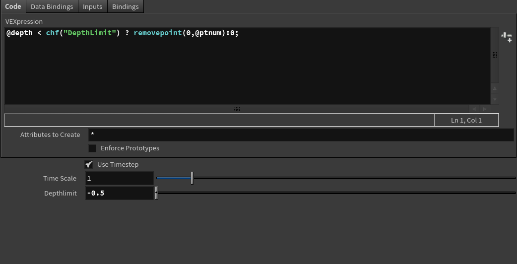
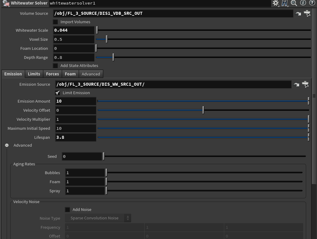
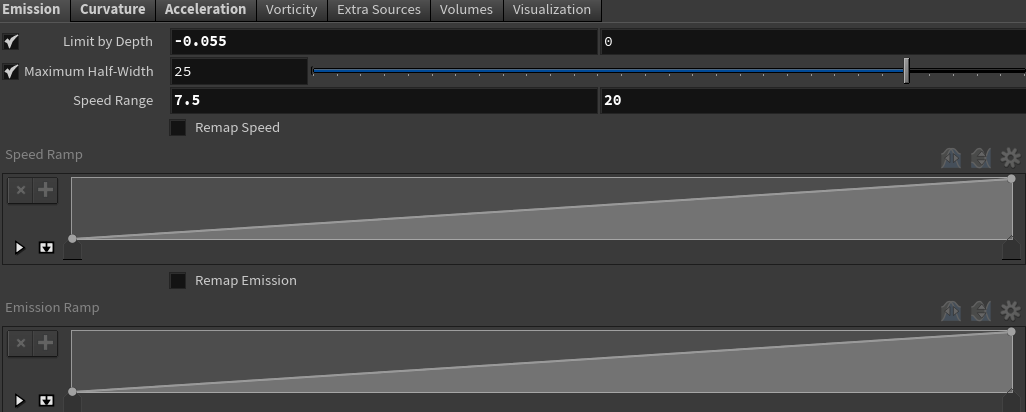
After the simulation, we could start to build the whitewater source. Basically, most of the whitewater comes from the flip surface field as well as the vel field, and they are not hidden inside the flip mesh. First, I have created a bounding box to select the area that needs to be imported for the whitewater simulation, then copy and transform it to generate multiple boxes with slight overlaps. (For the VDB combination and velocity information exchange) After that, It is unnecessary to keep the inside part of the whitewater source since they also create whitewater particles that slow down the simulation speed, so I imported the ocean surface collision volume to the sop solver connected with the whitewater solver, deleting those particles during the simulation. For the whitewater emission type, I only choose the “Acceleration” for now because it is directly affected by the vel field from the flip cache, and I could adjust the range based on velocity length under the emission tab. Finally, make sure the whitewater has the depth limit and collision with the bungalows also.
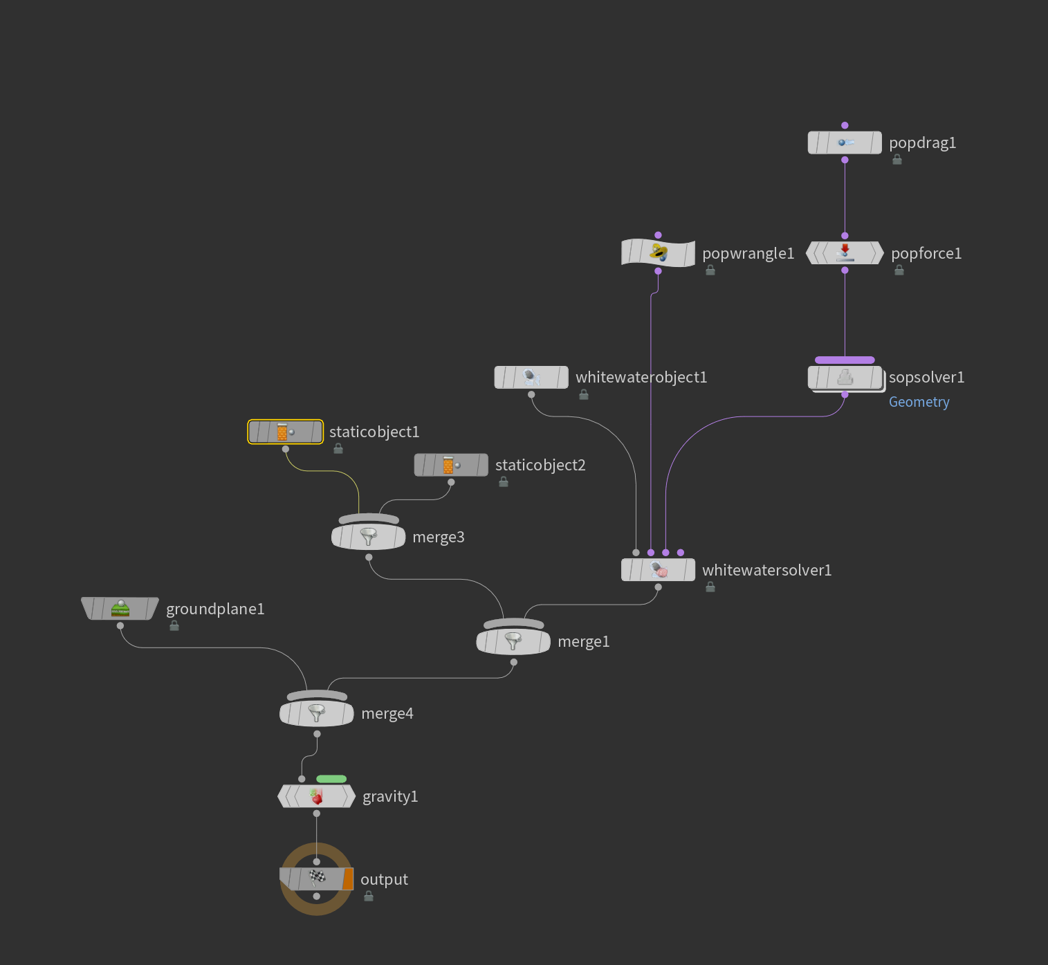
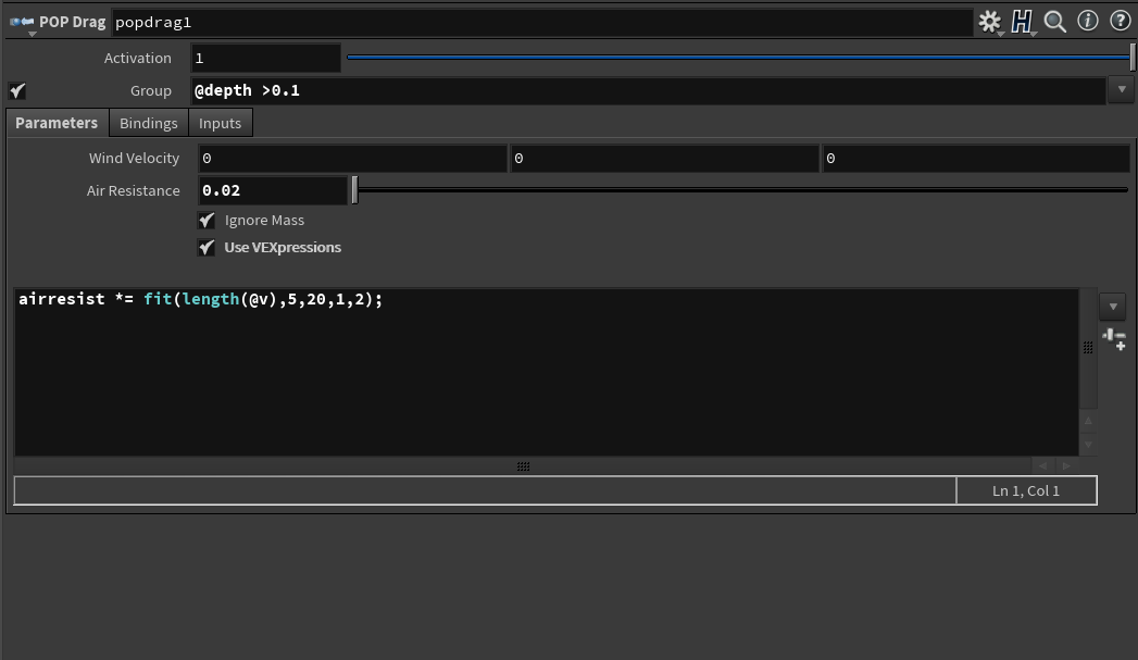
We could execute the same optimization process for the whitewater cache by keeping the age, depth, and velocity attribute only. Then the whitewater particles can be used for generating water mist. Mist has a larger spread range and higher air drag and finally rendered as a thin fog shape to increase the volume looks on the surface. Inside the mist simulation setup, most of the nodes are similar to the whitewater setup. However, there is a custom setting for inherited velocity from whitewater simulation. The Pop source node has a uniform velocity variance by default, but we could dive in the node and replace the parameter with our own one to override the parameter outside. (Based on velocity length) Also, the air resistance has been increased a lot and can be controlled by a ramp based on particle age attribute. The birth rates also need to be treated carefully depending on the machine performance limitation.
Mist sim in Shot 02
Custom Pop velocity inherit variance
After the mist simulation, we repeat the same optimization process and merge all the elements, and the result looks good for now. Mist has 6 million particles within a single bounding area, and whitewater reaches 20 million particles as well.
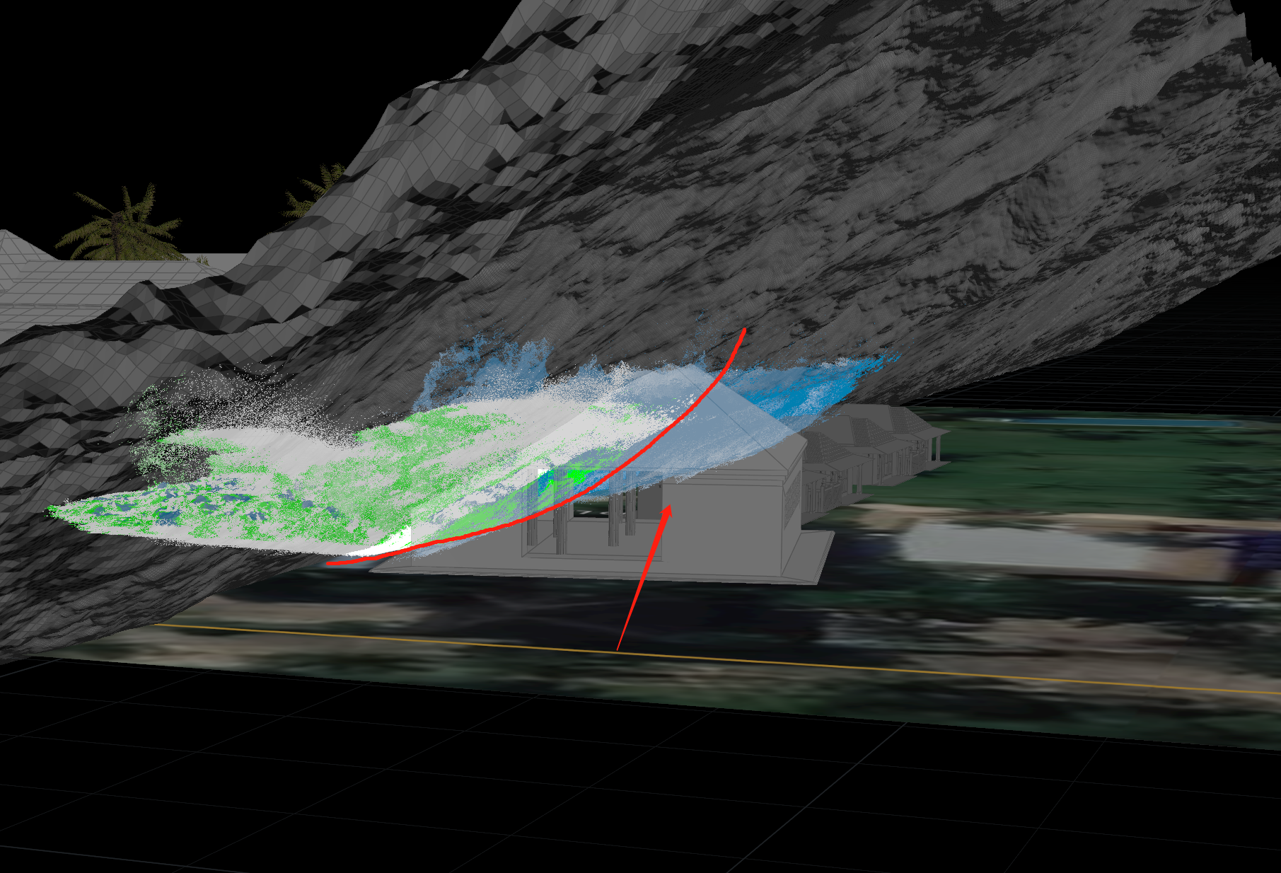
Flip sim + Whitewater sim + Mist sim in one bounding box area in Shot 02
Flip sim + Whitewater sim + Mist sim in one bounding box area in Shot 01
Update 04/25
(Modify the ocean surface)
(Modify the flip source on emission type and range)
(optimize cache size)
Based on the feedback for water dynamics, this week I start to modify the ocean surface a little more. Now the ocean spectrum only controls the noise details on the surface but not the animation. Also, the grid length has been extended to cover more areas inside the camera view.
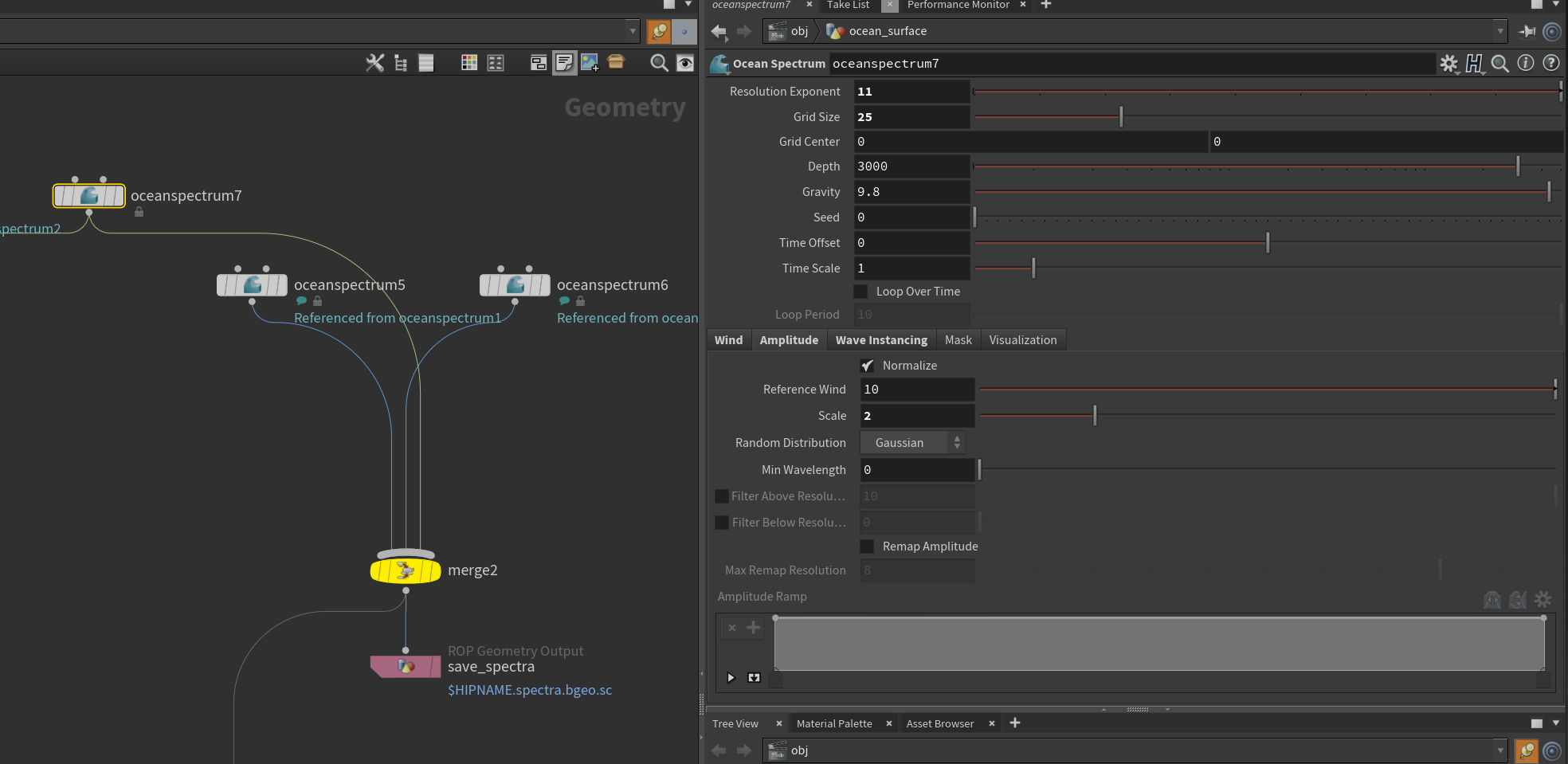
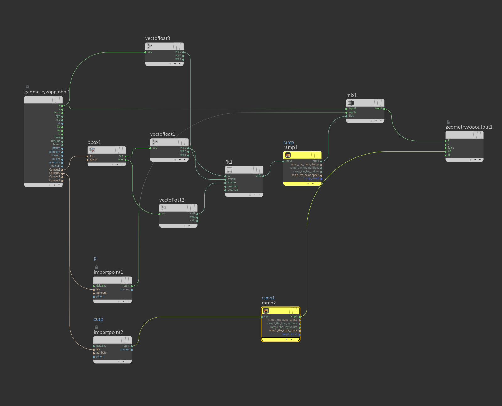
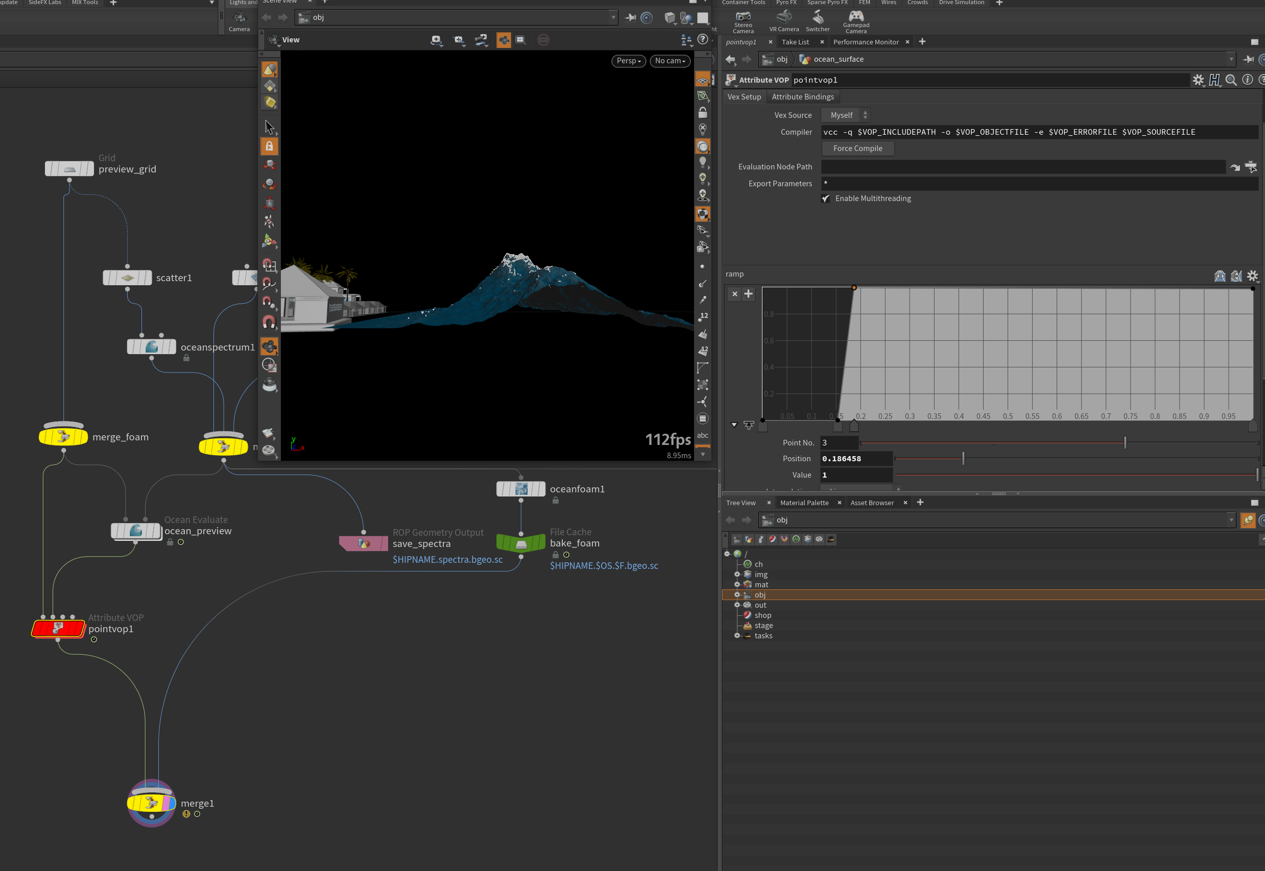
To adjust the wave height with more flexibility, I have calculated the bound of the grid and connected it to a ramp control. Now the height of the wave could be animated, so It would be more destructive when closed to the camera by increasing the value gradually. Meanwhile, using the “compile” node for caching process results for other node references is very efficient. The compile process only runs once and store the result, so it will not affect the loading speed while in reference using the “invoke” node. Here is the video demonstration for ocean surface customization.
Ocean displacement workflow
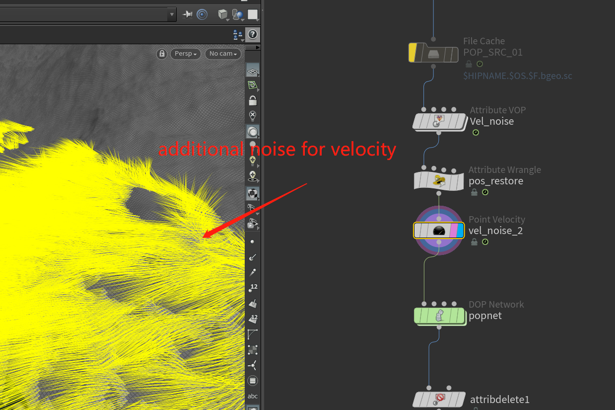
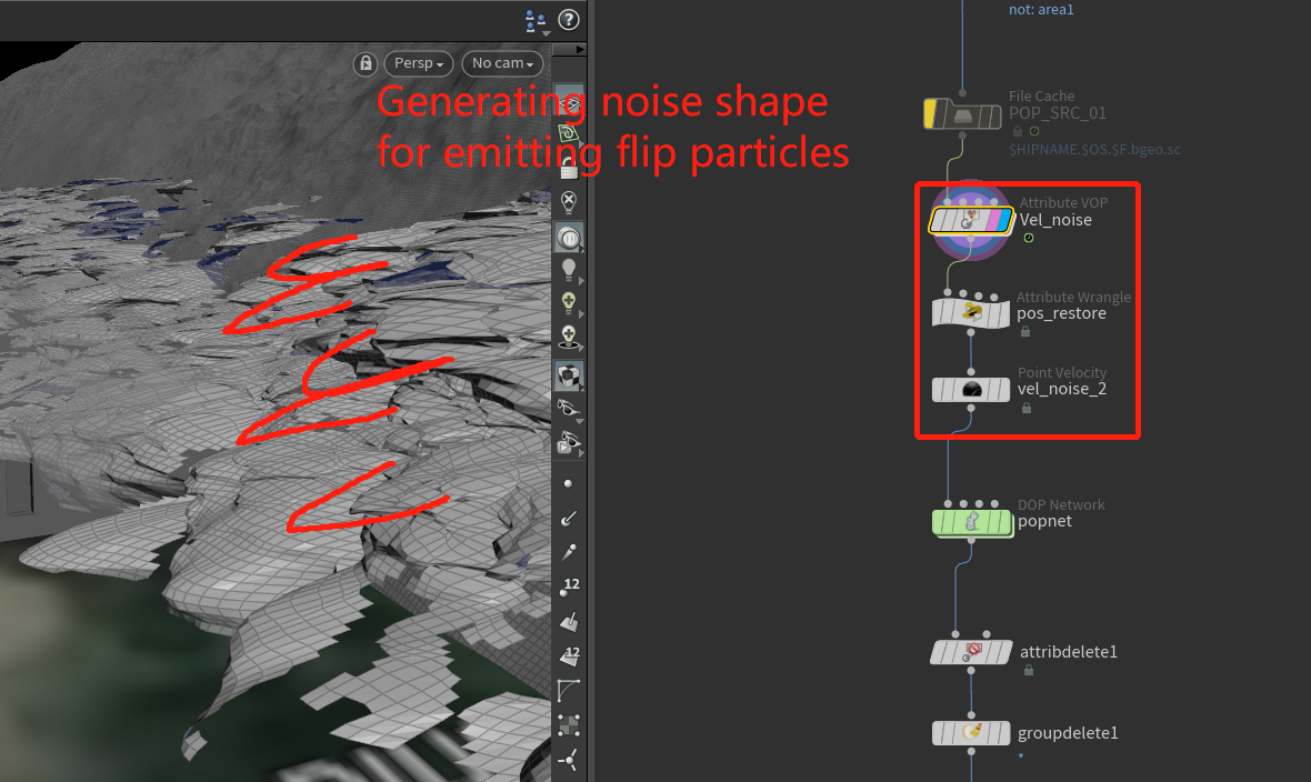
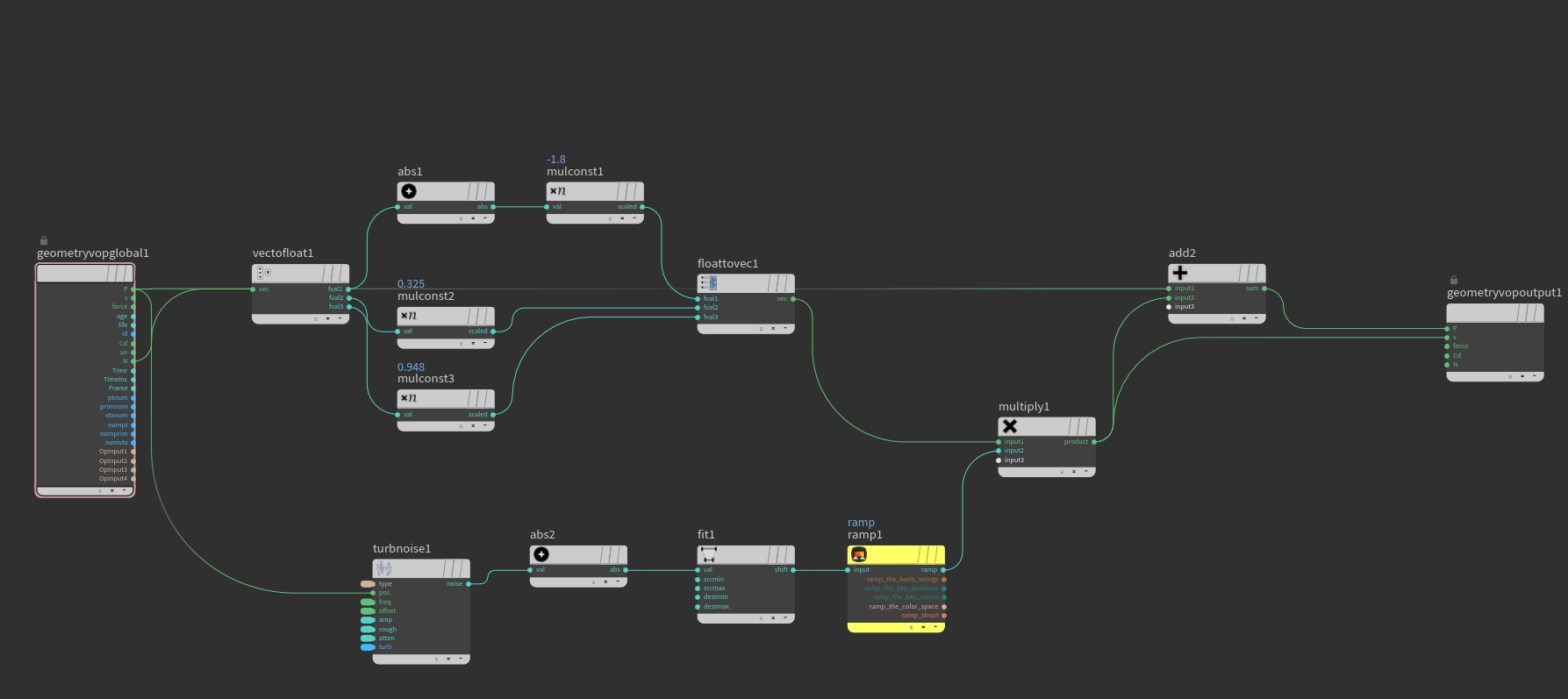
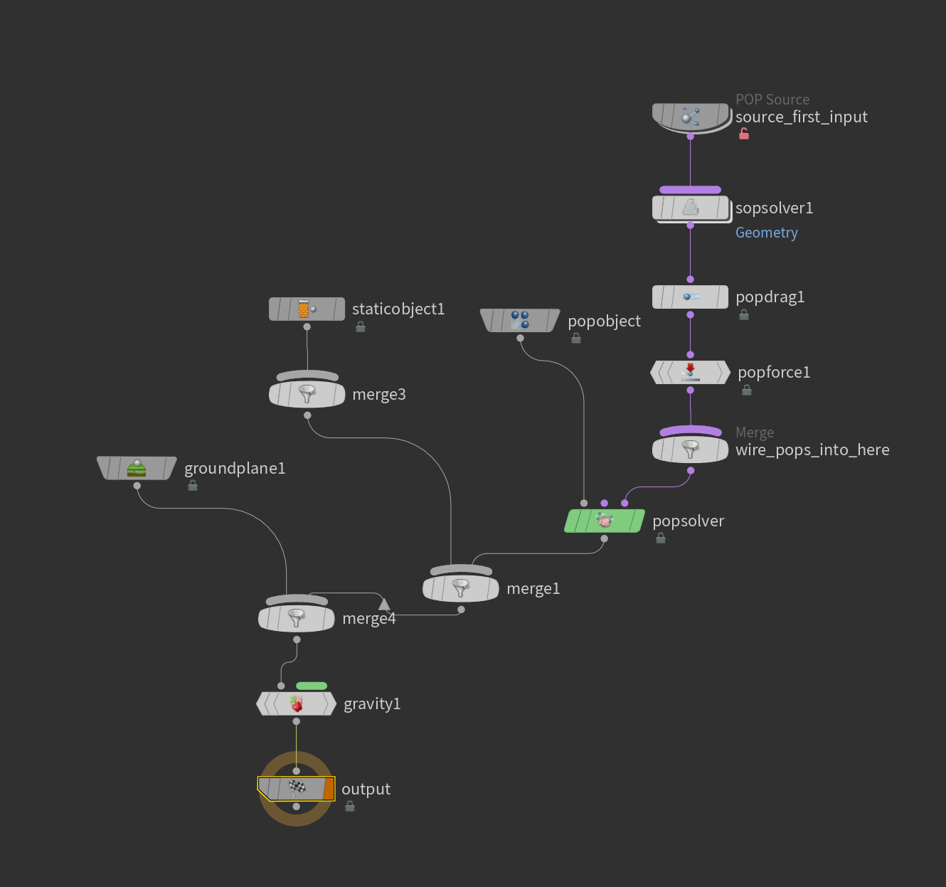
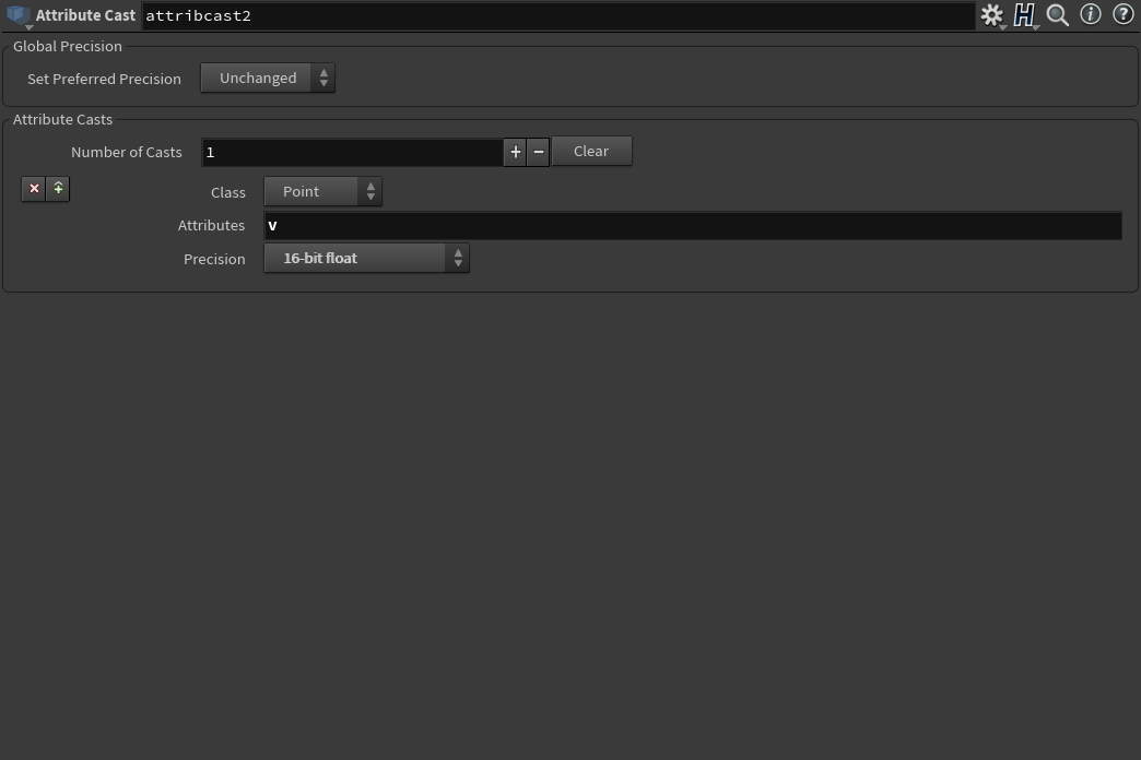
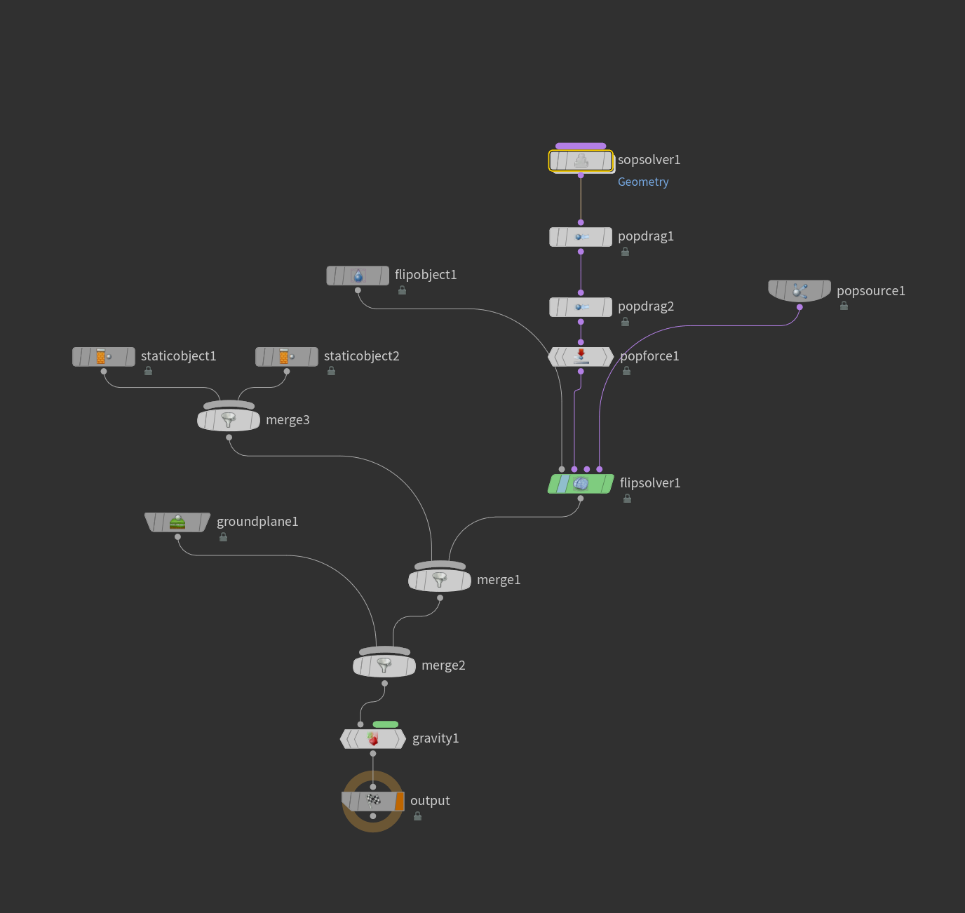
For the flip source, because the ocean surface has been extended, it will be heavy to simulate all particles at the same time (Last week’s simulation time is too long for iteration even it was just the flip particles), so I have decided to do separate flip test for speeding up purpose. First, I created a bounding box to cover parts of the pop source which is used for emitting flip particles later, and generated a random velocity before the source simulation. Then, since I have decided always to use the particles to emit fluid, the flip source now has more dynamics than the previous version (the flip source has the collision with the bungalows now). After that, I found a very useful node named “attribute cast,” which basically converts the attributes to a specific data type and thus saves lots of disk space, and I have used this node to convert the velocity of simulated filp source to 16-bit-float format.
For the flip simulation, I have imported the simulated flip source using the “pop source” node and set it to continue emitting from start to end to replace the previous emitting method. The “reseeding” function has been enabled to prevent particle density drops in high-speed areas and use the sop solver to delete intersecting flip particles with collision volume. And the velocity smoothness has been lowered down to ensure the splashes have more details when colliding with the VDB proxy.
Update: 04/17
(Continue on water simulation)
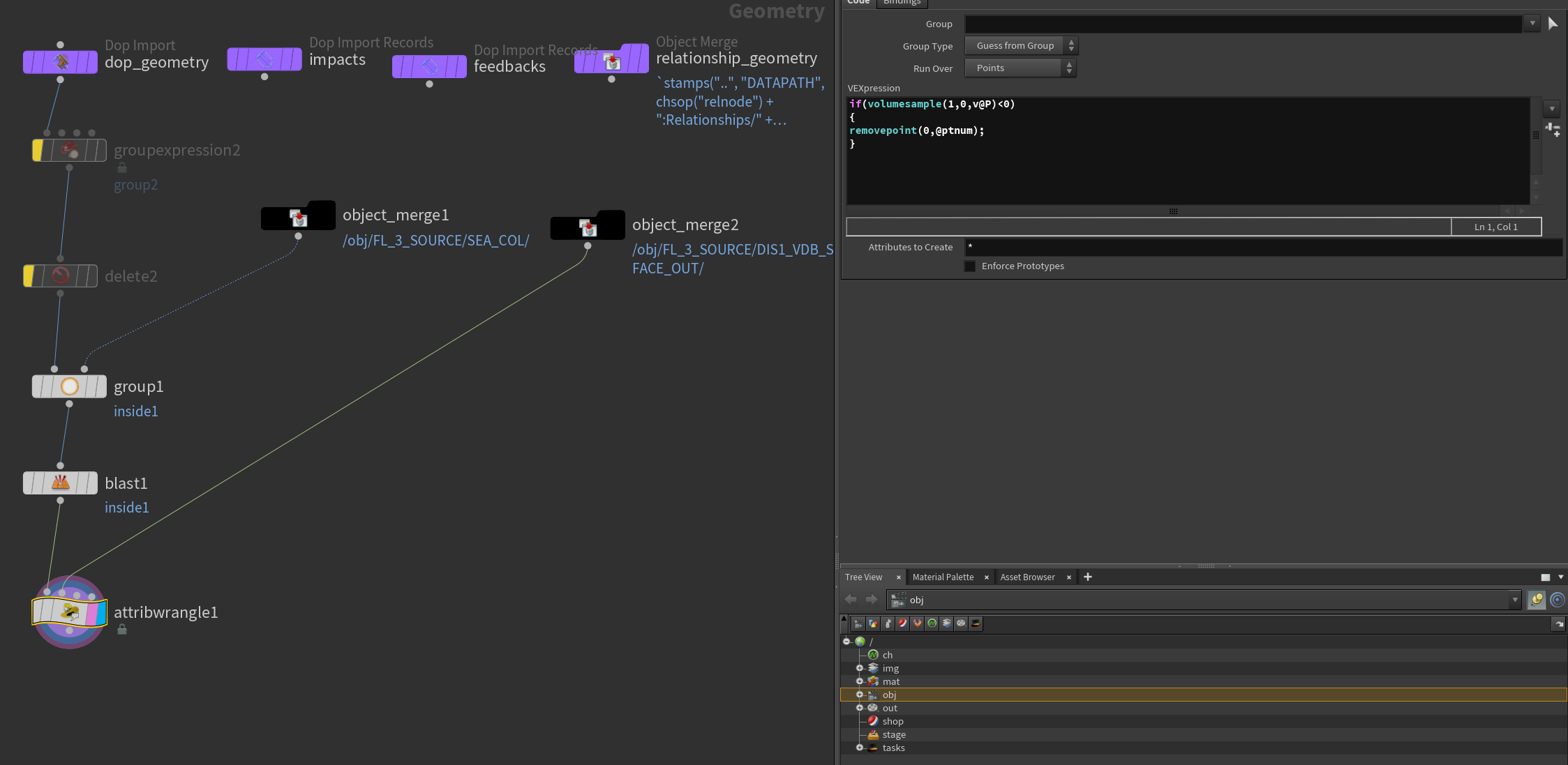
This week I started to replace the previous emitter for the splashes and run the sim with different parameters. From last week’s feedback, I have gained lots of efficient methods to limit the speed of flip particles, which helped the progress a lot. The ocean foam source node has been switch to the “emitter” mode to generate the flip source right now. Since it is all points with velocity inherited from the ocean spectrum, the only thing before transforming them into the flip source is to convert them to VDB, which ensures the necessary fields to be generated. After that, using the “clip” node to delete some parts below the ground plane and it is ready for the source. For the collision geometry, what I wish to achieve is that those flip particles emitted by the source should have collision behaviors with the ocean surface. So I have tried both ways: the volume collision source and using static object collision with VDB proxy. Both worked fine but the dynamics looked different. Also, the sim time of volume collision source is slightly longer than the “static object” method, but it has more splashes dynamics.
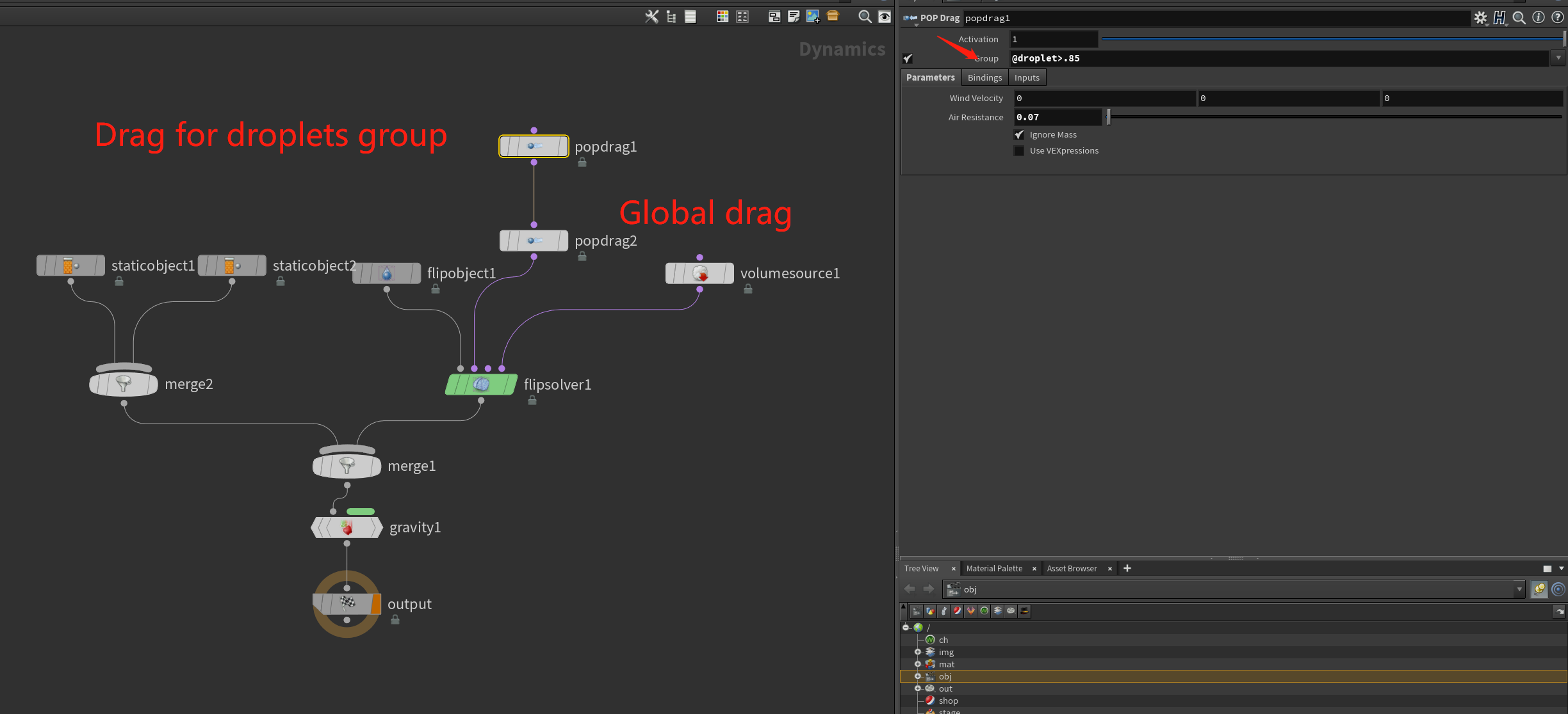
Also, the speed limit node is another way for limiting maximum particle speed based on groups. Since the droplet group has been enabled inside the flipsolver, I could separate them and only applied the node to the group without affecting other particles. The maximum speed value can be adjusted according to the camera view. For the second closed-up shot, the max speed for droplets reaches 4 and it seems the number still needs to be increased for a better result.
To blend the front of the ocean spectrum to the ground plane I have a custom point vop node to control the displacement based on the primary direction distance so the front would stay flat but others remain the same displacement value. After that, I could use the flip simulation to cover those areas to prevent overlapping.
Update 04/10
(Start to add props to the scene)
(Ocean Wave test / Splashes test)
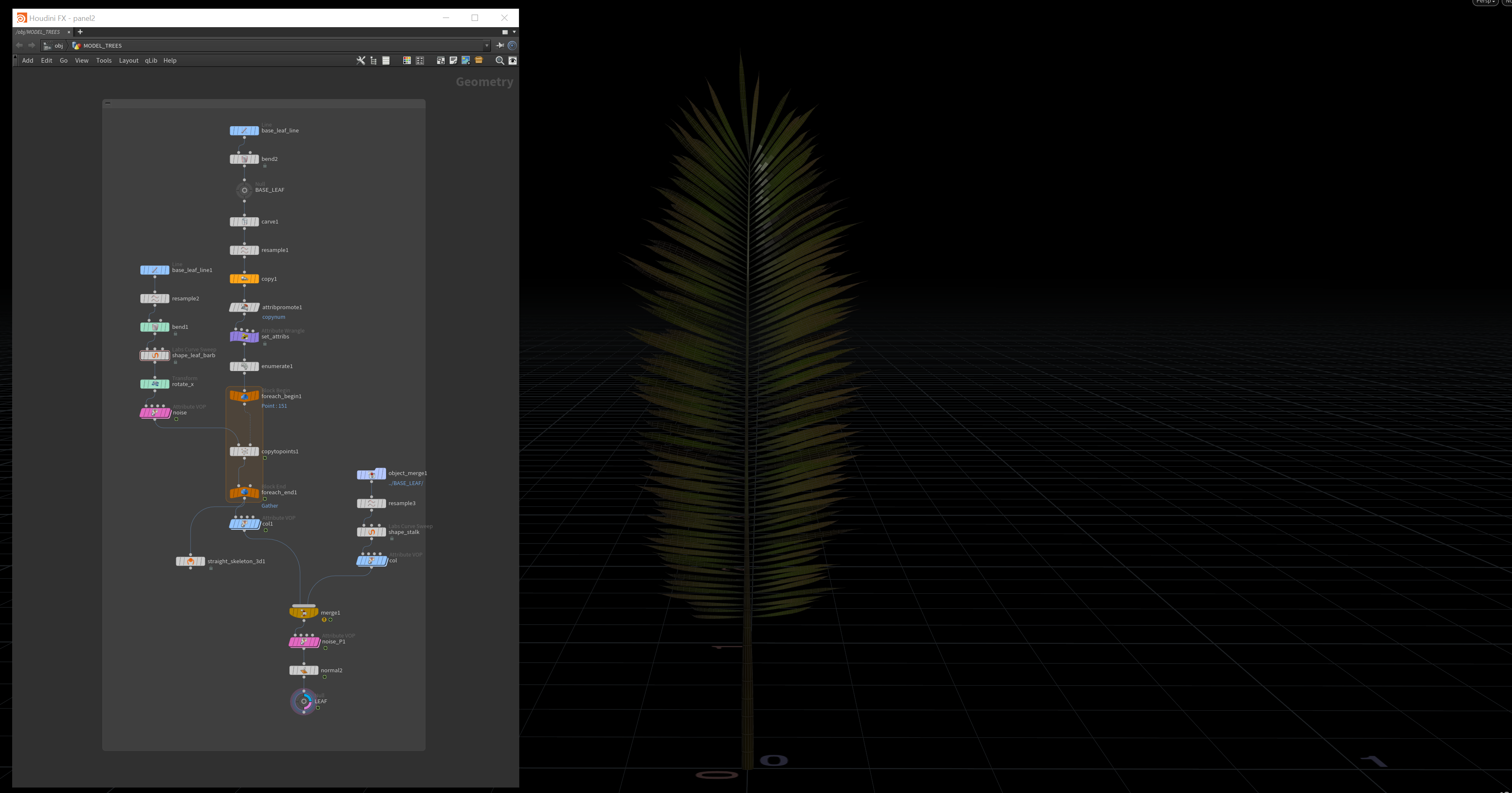
The resort building draft is almost finished, and it is time to add palm trees and other small props such as beach umbrellas and table sets to the scene. For the palm tree model, using PDG to generate multiple variations saves much time for randomization. The palm tree is modeled inside Houdini, while some parameters like height and bend can be promoted to up-level for PDG to wedge. Later, the tree model will be rigged using skeleton curves generated by the KineFx node to simulate water influence.
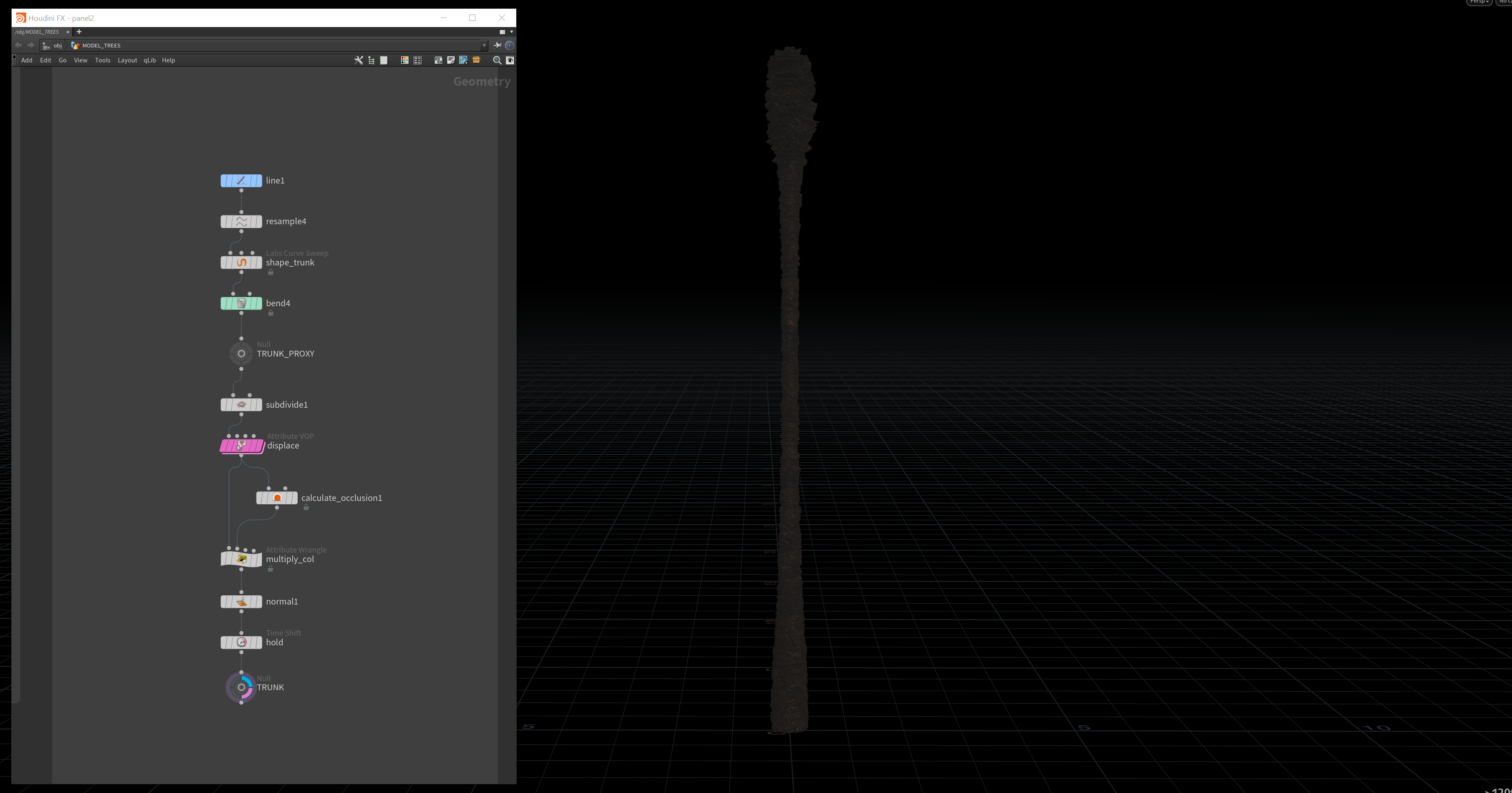
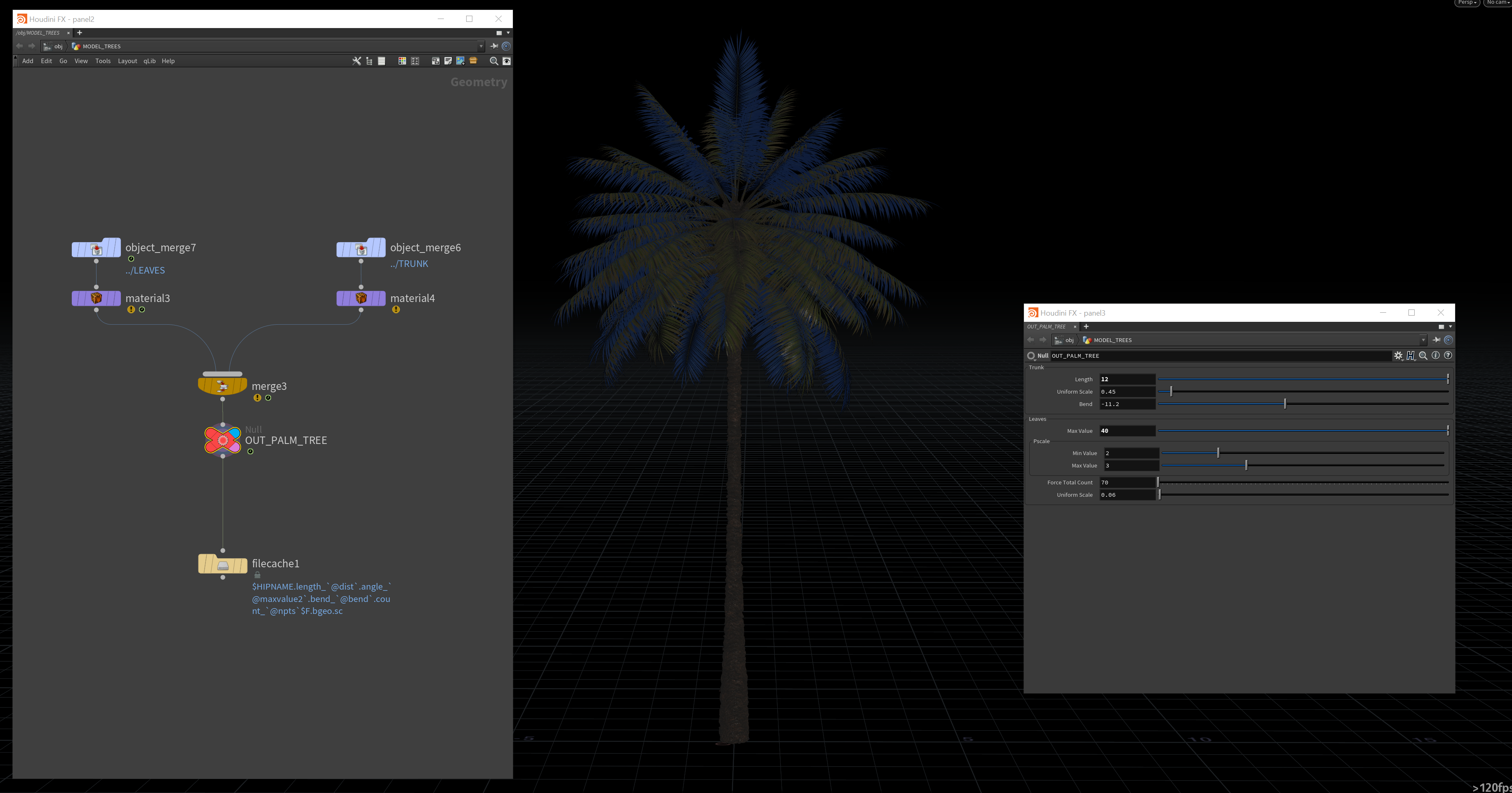
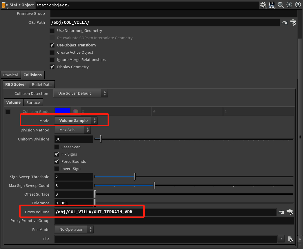
For the splash simulation test, a box filled with points is a good start, then turn them into the flip source with noise applied. Inside the Dop network, since the villa model has high polygon counts, they need to be converted to VDB proxy before the flip simulation. The flip source for the water splashes test is almost 25 meters wide compared to the scene scale. Moreover, the max particle count for the splashes simulation reaches approximately 18 million. (Particle Separation at 0.028 with reseeding off). Here are some tests varying parameters like "Grid Scale", "Velocity Smoothing," etc.
Splashes playblast
What influences the dynamics most is the "Grid Scale" parameter. The default number for that parameter is 2, which is the most common usage value. When the value is decreased to 1.5, the simulation cannot maintain dynamics with high-velocity splashes with the same amount of particles since this parameter controls the grid definition in voxels. Here is an excellent explanation about how the "grid scale" actually works: https://www.sidefx.com/forum/topic/60343/
Also, to slow down the droplet's velocity in the air, drags depending on the droplet group have been separated to global drag to avoid particles glitch in some areas. Those values depend on particle speed so that they could be adjusted based on shots requirement.
Issue: the ground surface friction seems not to affect the behavior of the flip particles. The ground surface has already been extruded and converted to VDB Proxy. but the collision detection works fine. What I want to achieve is the flip particles start with high velocity and then the velocity dissipate with the time factor.
Solution: Thanks to Dale Bunten and Professor Fowler mentioned increasing the friction parameter to an extreme level around 50,000 and 100,000 to see if that affects the particles. Also the ground might be too flat since it is just a simple plain without any terrian noise.
The ocean wave simulation right now is based on ocean-guided simulation. The flat tank received the ocean spectrum information from VDB conversion. Multiple fields have been separated, such as surface vector field and velocity field. The flip solver will read that information using the Gas Guiding Volume node. The second one has the boundary keyframed to ensure the wave moving forward without clipping.
Update: 04/02
(Continue with the resort building and add more cams into the scene)
(Ocean Spectrum test)
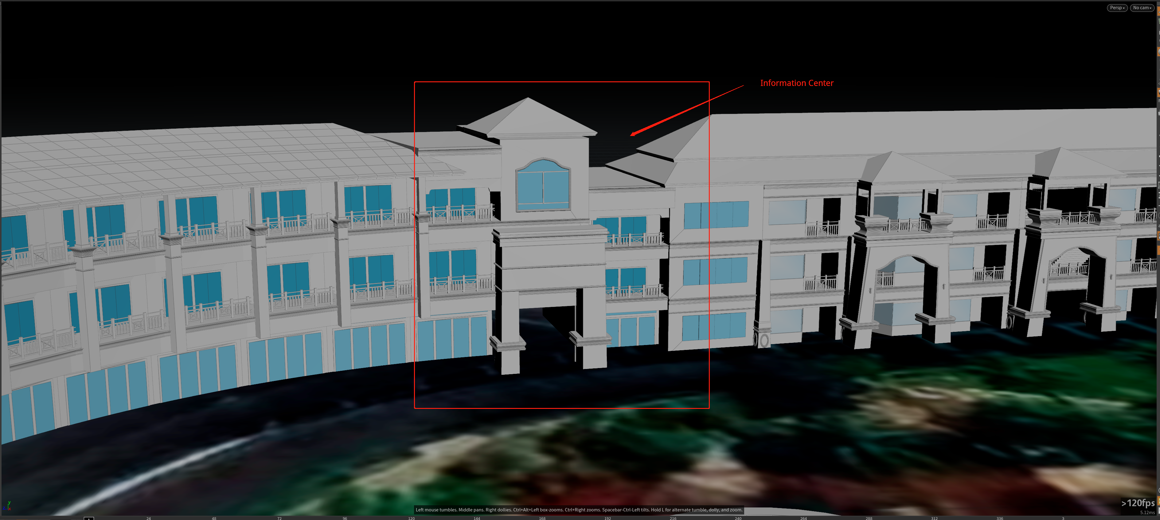
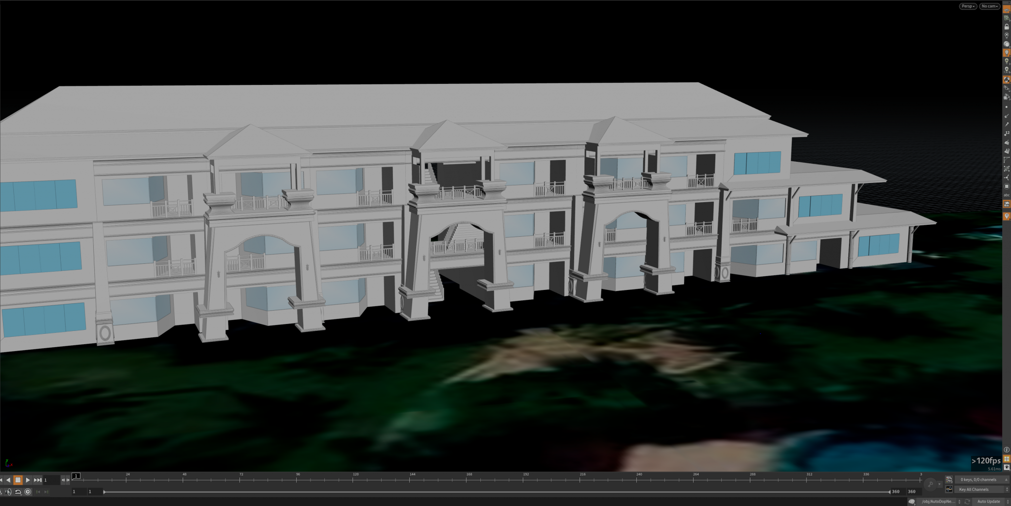
The main building of the resort is nearly finished and one more part is still in the progress. From the satellite view, the main building has a curved shape in general. To achieve the same look, the model need to be deform by a curve manually using “bend” node, so the model can be driven to the direction which is similar. Notice that the “information center” part is a little different than others so it has to be modeled individually and thus act as a connected portion from left to right. The whole environment still need props and trees placed in the middle area.
Another camera was created in a low perspective near the ground to ensure a wide-angle look for the coming ocean. This could be the first shot showing the impact on those bungalows. For the ocean spectrum that displaces the ocean surface, two separate “ocean spectrum” nodes were layered to maintain details when the water approaching near the camera. Right now the wave height is approximately 25 meters above the ground and the speed is about 20.8 km/h in the direction.
Also, use the “ocean foam” node to generate the white cap and streak look when rendering the ocean surface, since the default ocean shader recognized the foam as a volumetric object so the foam looks depending on the shader tweaks.
And here is the first render test with ocean shader, the environment only has one HDR attached. Be careful with the "Displace Bound" value since it basically decides the maximum displacement can reach in the final render. The default value is not enough for this case so increasing this value about nearly the same with the max wave height could actually works.
Update 03/24:
(Start to build the resort environment)
The building on the right side is nearly finished, as some small details may still need to be reworked. Going to model the front side of the resort building, most of the structures are pretty same so the copy function should works. Also, one camera for the large angle shot has been put into the scene to check the resolution and safe zone for the scene. The position has not been decided yet as it is just for the test purpose. Might do another cam of angle if it is required.
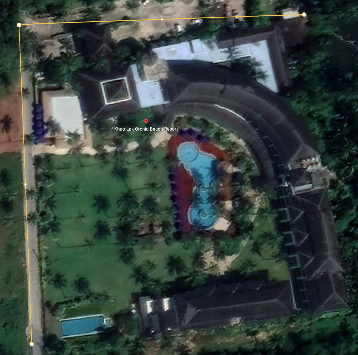
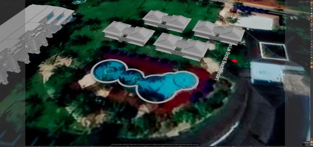
One top view from Google Map of that specific area has been used for scale reference – the name for that resort is “Khao lak orchid ” which is located in Khao Lak, Thailand. The actual location can be found here: http://www.khaolakorchid.com/ https://www.google.com/maps/place/Khao+Lak+Orchid+Beach+Resort/@8.6851491,98.2393274,17z/data=!3m1!4b1!4m8!3m7!1s0x3050e96b6ec7f6eb:0x85bd2c42b81ee22b!5m2!4m1!1i2!8m2!3d8.6851491!4d98.2415161
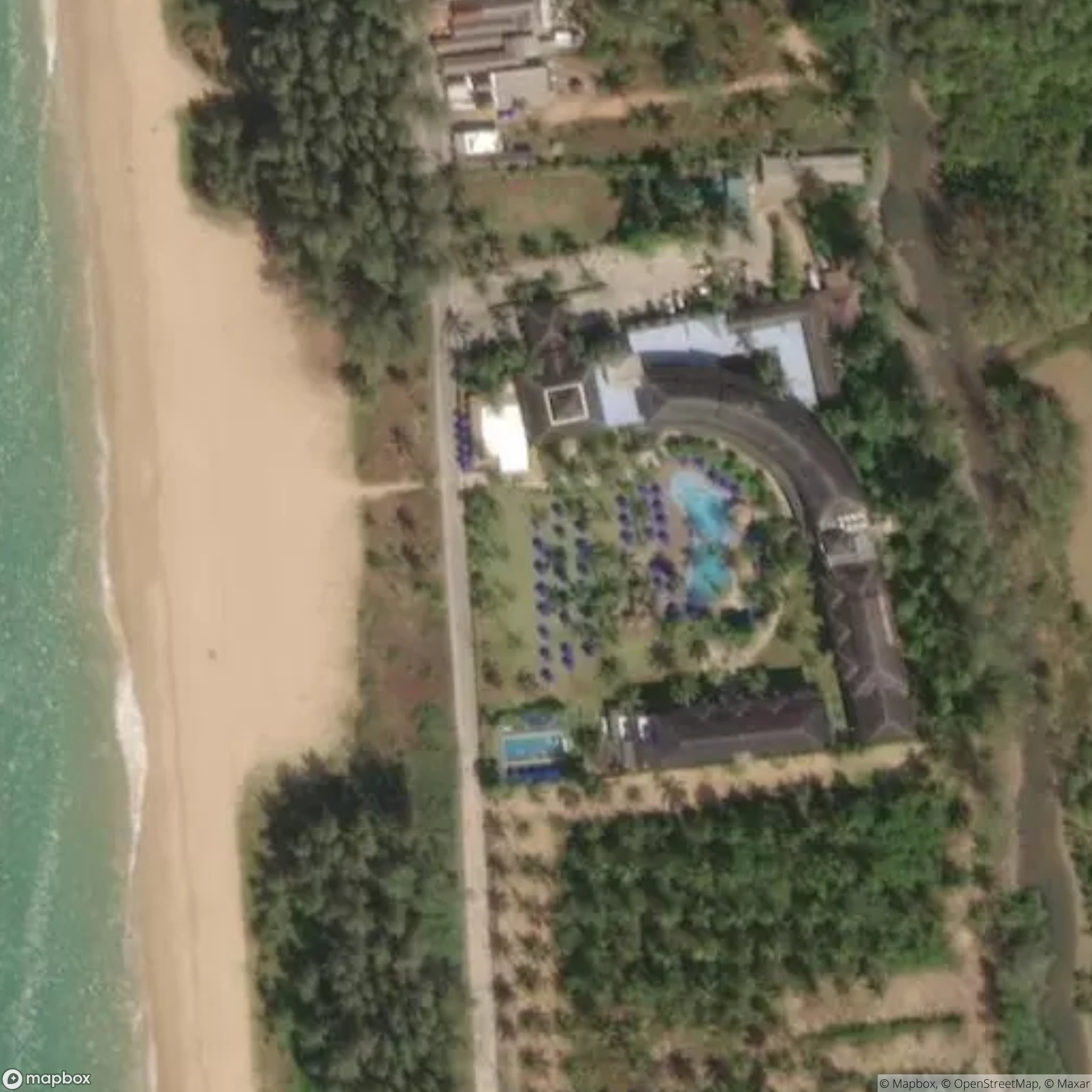
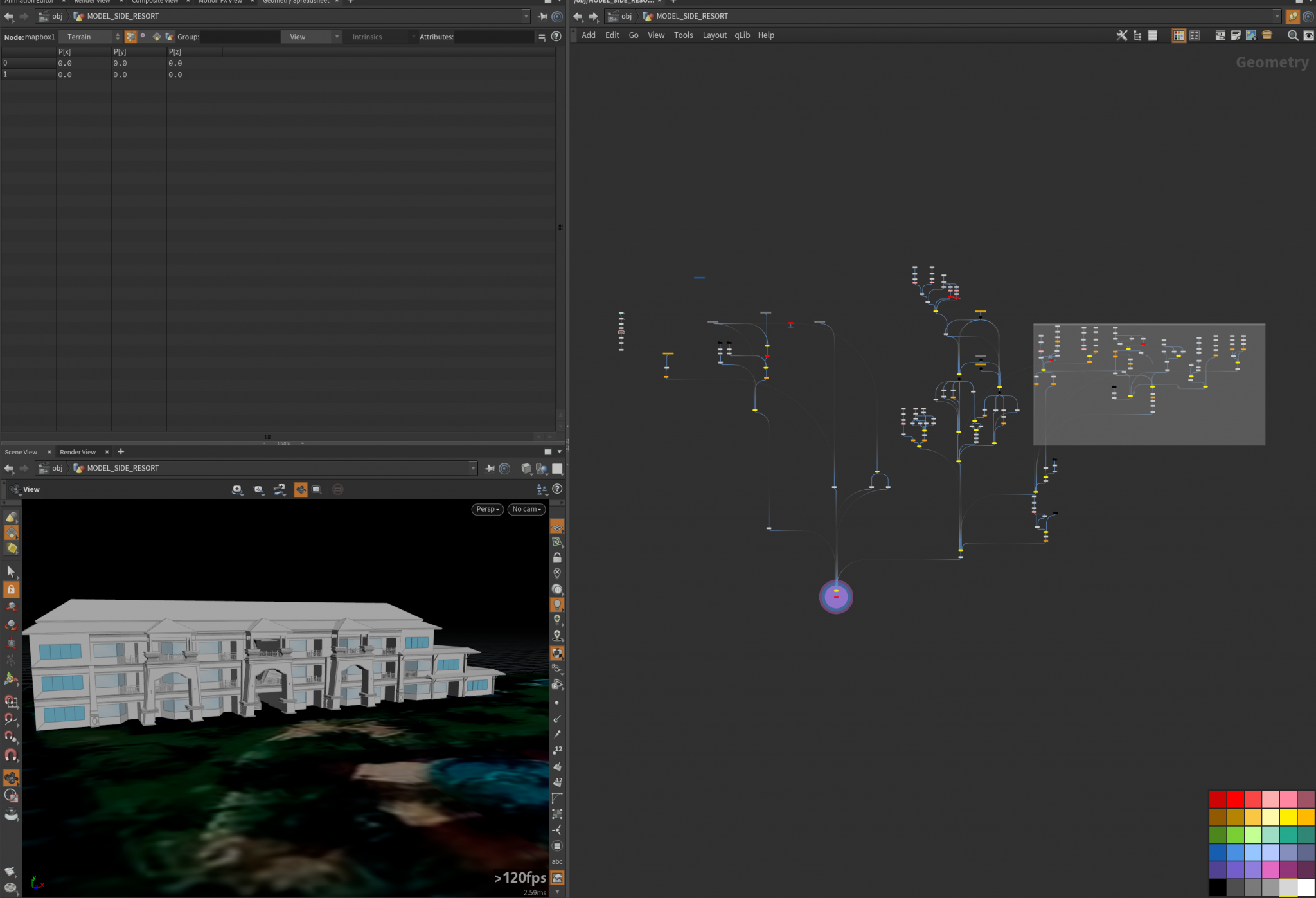
Also, the satellite data from Mapbox has been imported into Labs Mapbox to generate a basic 3d model representing the depth of heightfield.
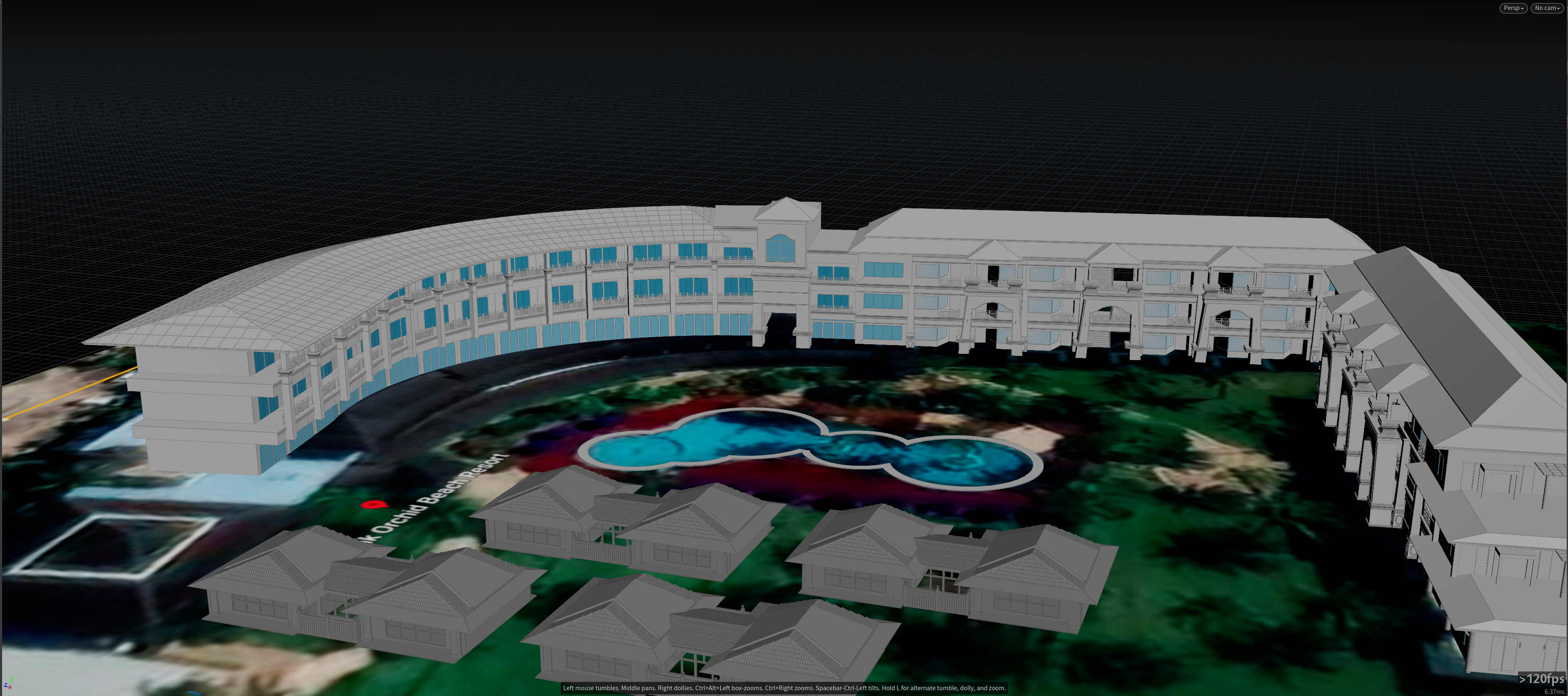
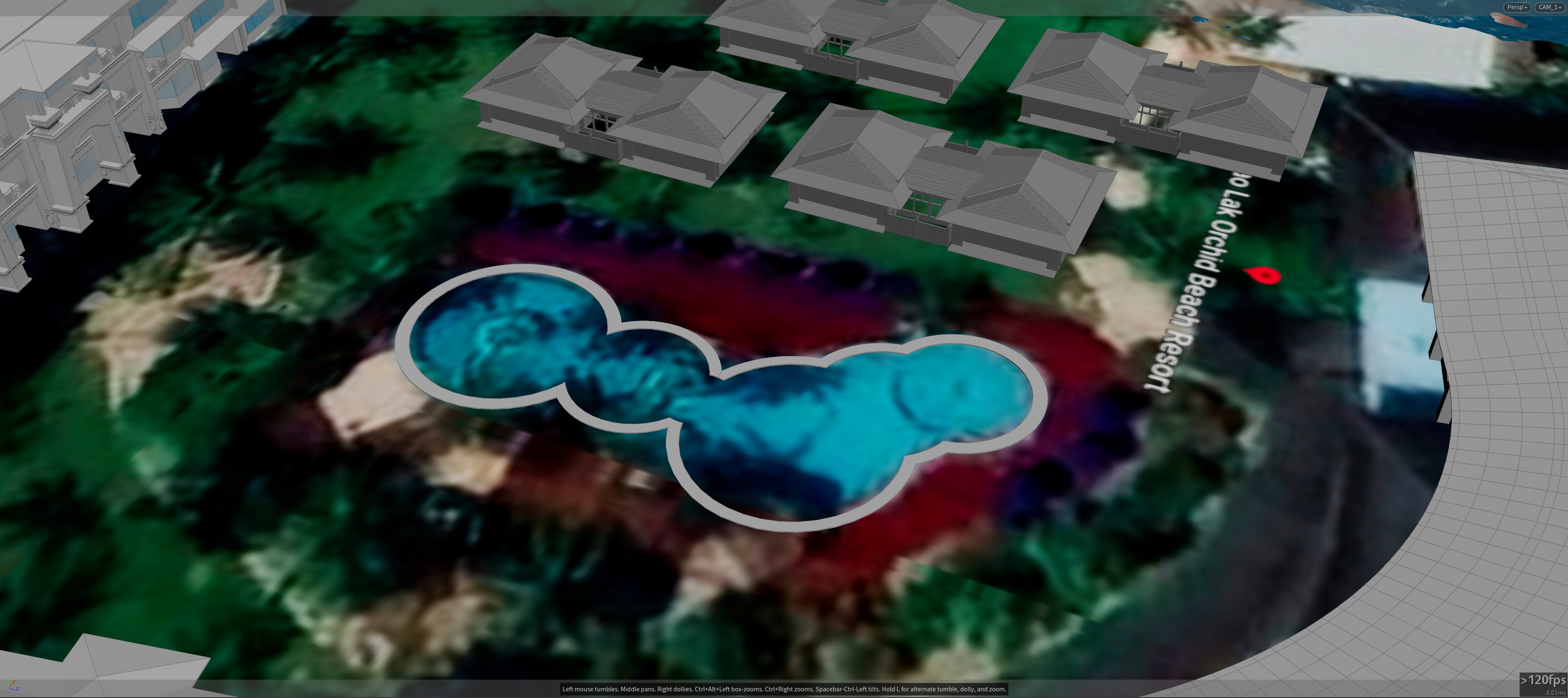
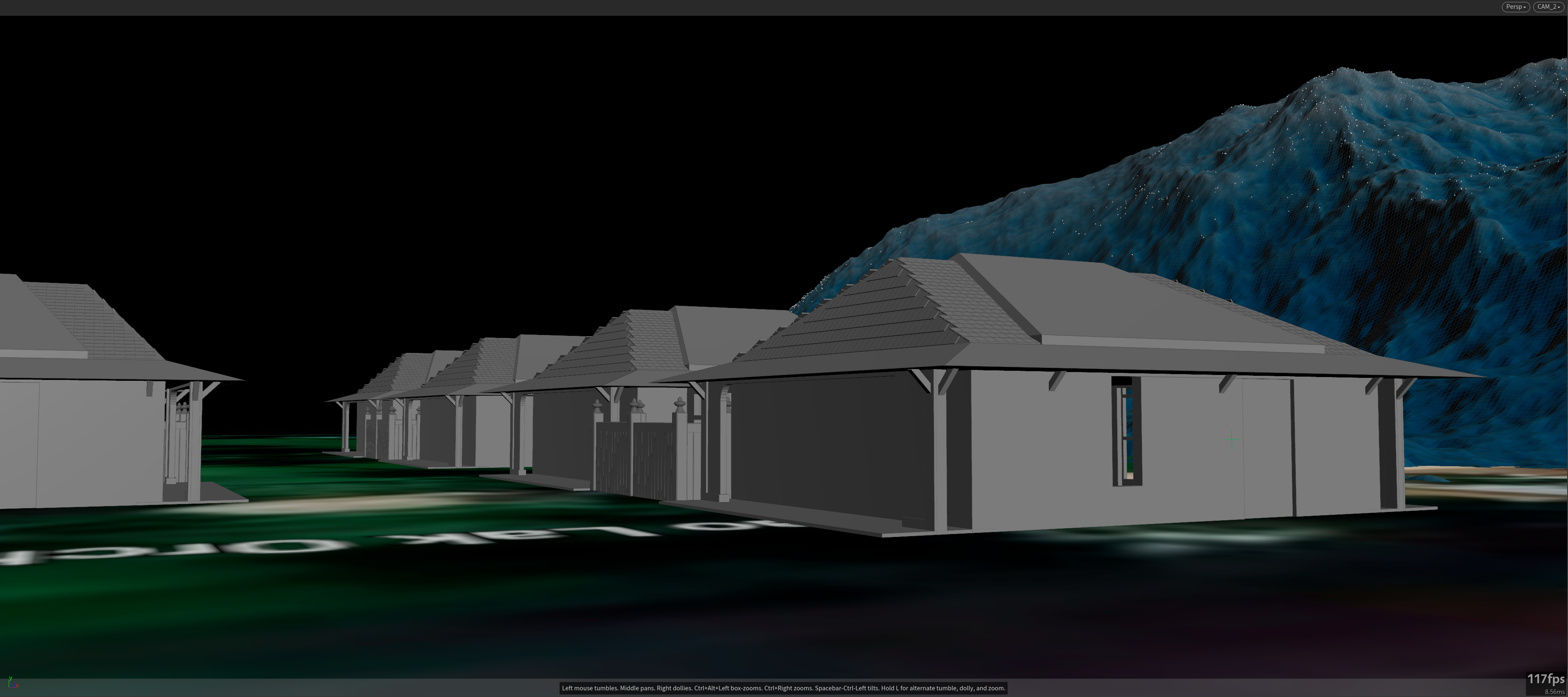
First I have modeled the bungalows near the road, which could be the first impact section on the resort. Those models are carefully placed at the location since they are actually not existed in the satellite map.
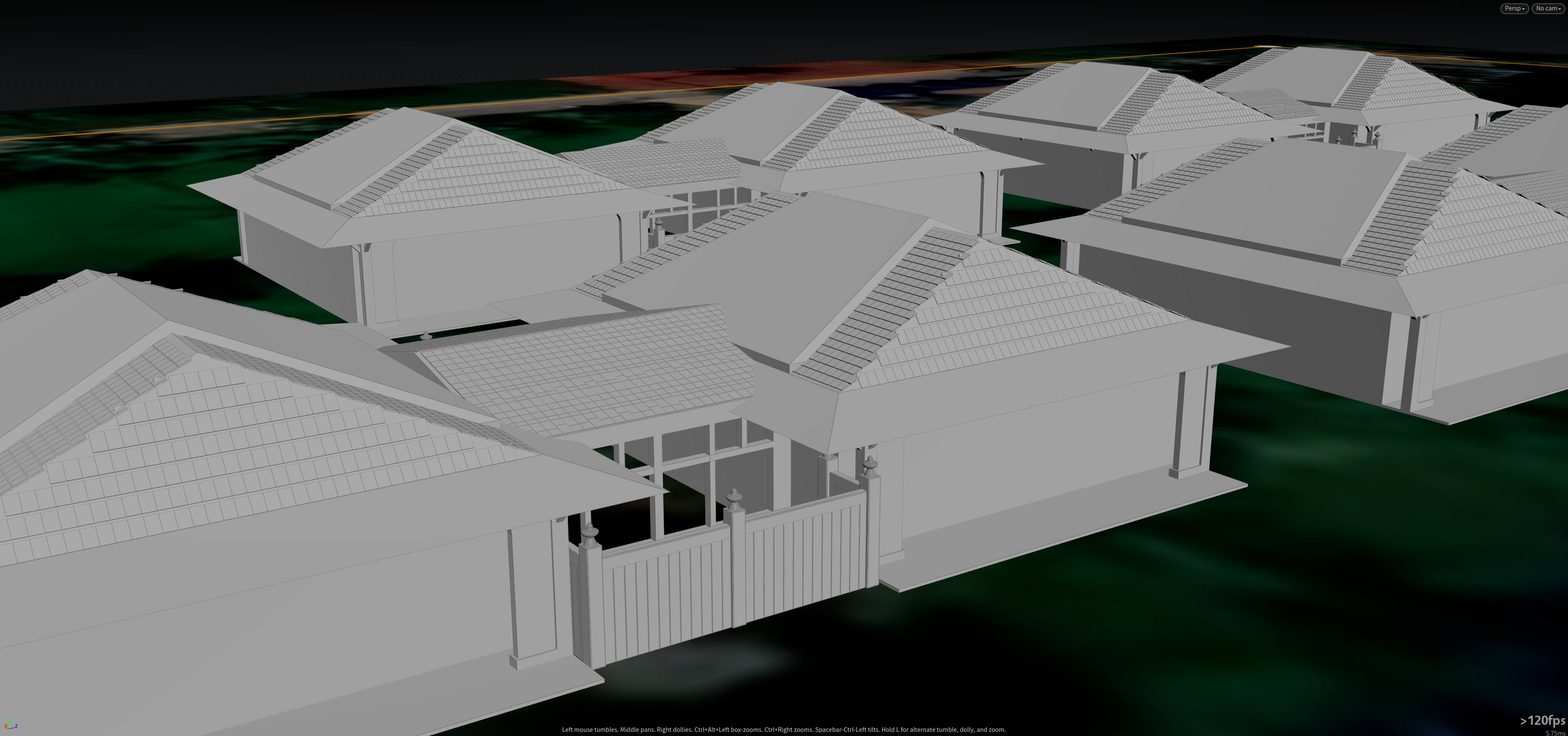
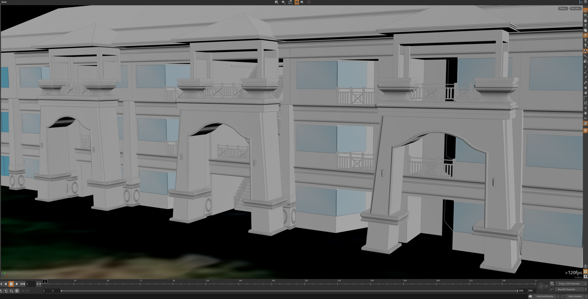
After that, I started to build the right side of the resort. The reference images I found online are from different angles so it adds difficulty for the modeling. For the three main entrance doors, I use the curve tool for outline shape and other parts are basic modeling with copy node and some procedural techniques.
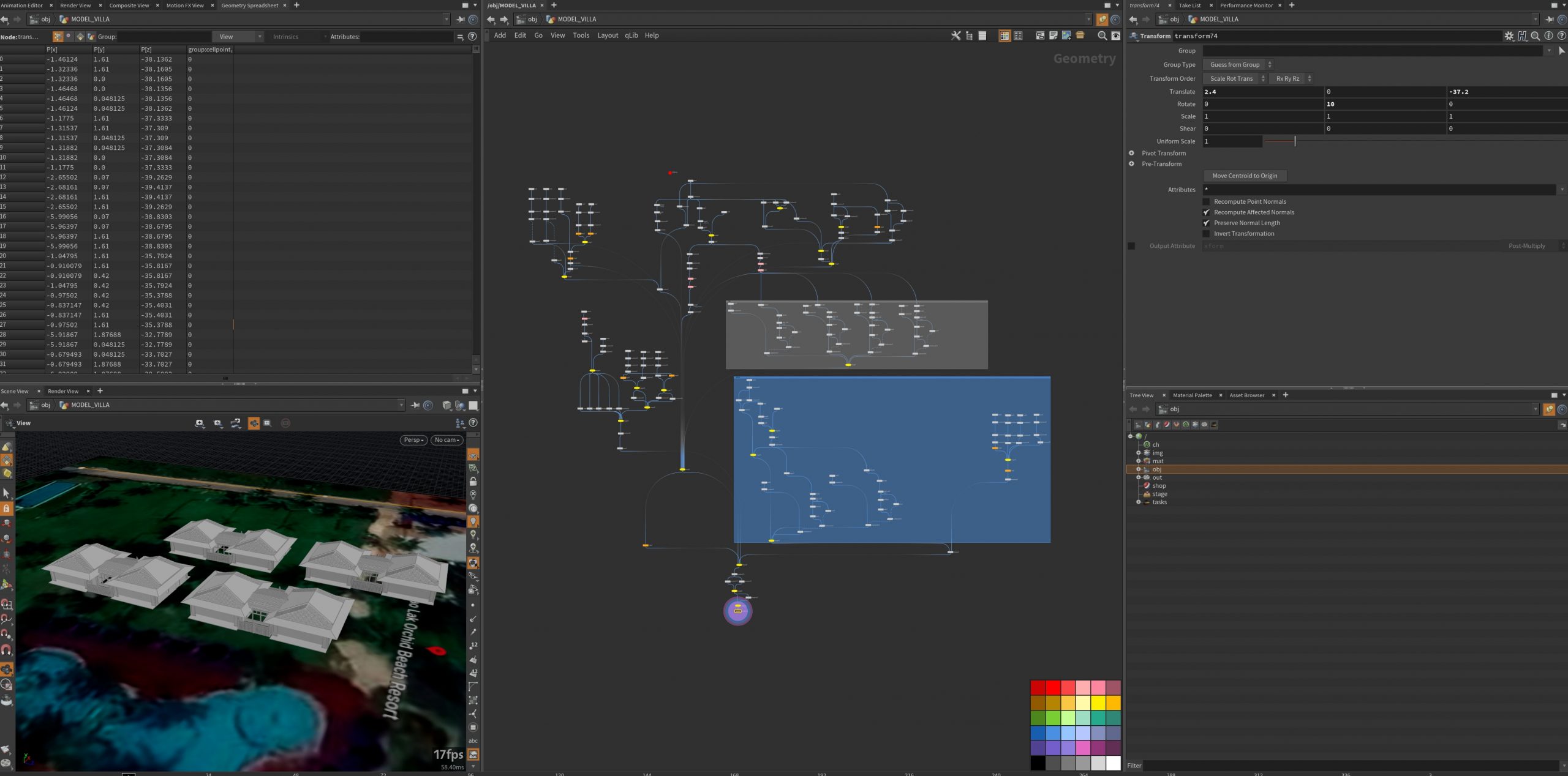
From the camera perspective, the models are going to be placed like this:
For the heightfield, using the “Labs mapbox” node to connect Mapbox API is necessary for generating the depth data. Since the resolution is not ultra-high, the depth map that directly created from that node would not quite suitable for simulation but I added a smooth node after that to ensure a sloped shape:
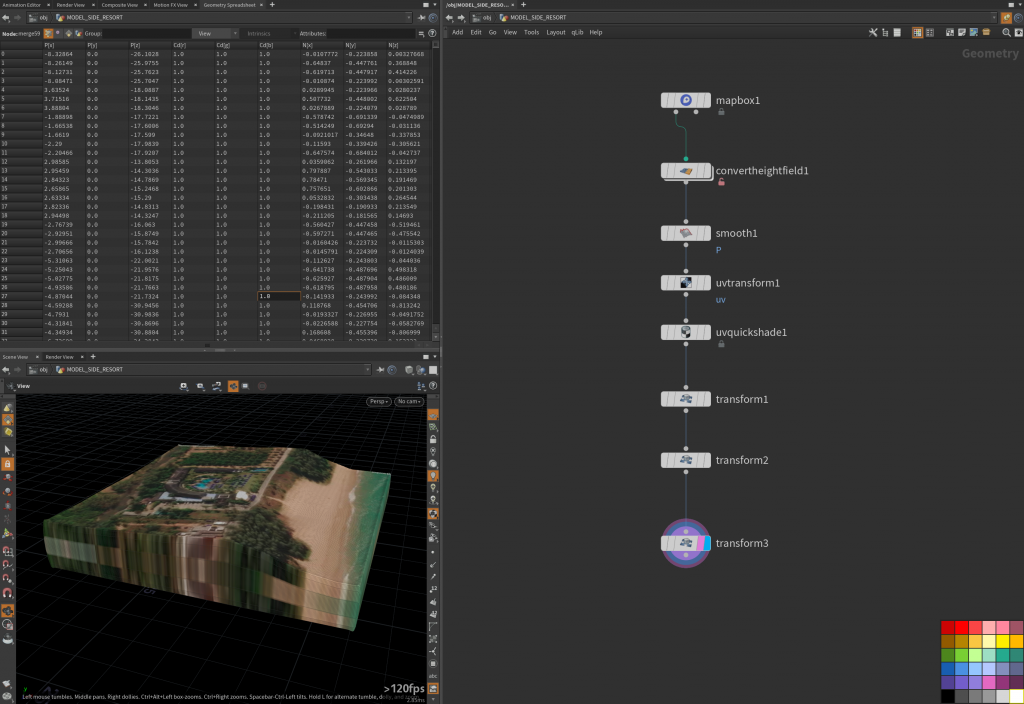
so after the whole resort model finished, it will be placed at the heightfield geometry to ensure it owns the correct depth above sea level.

